12 Monitoring Protocols
12.1 Introduction
This chapter describes statistical sampling design, data collection techniques, and analysis methods for quantifiable parameters to determine success of roadside revegetation projects. It is written specifically for field personnel as a quick guide to monitoring roadsides. It is not intended to teach statistics or explain the statistical basis behind the procedures addressed in this section. If the reader wishes to explore the statistics used in this chapter, a supplemental report (Kern 2007) details the statistical basis for each procedure. There are many approaches to statistically monitoring roadside vegetation. This report takes the approach that if monitoring is not simple, inexpensive, and objective-based, it will not be done well, or done at all.
The reader will be directed to those sections necessary to prepare and implement a monitoring plan. Three questions must be to answered before monitoring begins:
- What are you monitoring?
- What is the shape of the sampling area?
- What is the objective behind monitoring?
The answers to these questions will lead the reader to different parts of the chapter (Figure 12.1). This chapter presents methods to record, summarize, and analyze data using the Excel® spreadsheet program. You can create your own spreadsheet, or obtain a monitoring Excel® workbook which contains the spreadsheets shown in the chapter by contacting the authors of the report. Before using the spreadsheets, the reader is advised to see whether the Analysis ToolPak is installed. If it is not, many of the spreadsheets will not function properly. To do this, go to the toolbar and select Tools, Add-Ins, then make sure that the box next to Analysis ToolPak is checked.
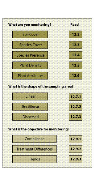 |
What are you monitoring? There are many revegetation parameters that can be monitored. In this chapter, parameters are grouped into 5 categories based on the following revegetation objectives:
- Soil cover — to determine whether treatments increased soil cover for erosion control.
- Species cover — to determine whether treatments increased native grass and forb cover.
- Species presence — to determine whether there was an increase in the number of seeded native grass and forb species.
- Plant density — to determine how many seedlings or cuttings became established after planting to assess whether stocking is adequate or the site needs replanting. Plant survival can also be determined from this protocol.
- Plant attributes — to determine how fast planted shrubs and trees are growing.
The procedures for monitoring each of these parameters are described in Sections 12.2 through 12.6. Each protocol discusses how transects and quadrats (or plots) are located, methods for collecting data at each plot, and how data is summarized for statistical analysis.
What is the shape of the sampling area? Revegetation projects associated with road construction can be classified into three broad sampling design categories based on the spatial features of the sampling unit:
- Linear areas — associated with cut slopes, fill slopes, and abandoned roads
- Rectilinear areas — associated with staging areas and material stock piles
- Dispersed areas — associated with planting islands, planting pockets, clump plantings
Each of these sampling designs has a set of procedures defining how transects and quadrats will be laid out. Section 12.8 guides the reader through methods for determining how many transects and quadrats to establish.
What is the objective behind monitoring? There are three basic reasons for statistical monitoring:
- Compliance — were regulatory standards or project objectives met?
- Treatment differences — are there differences between revegetation treatments?
- Trends — what degree of change is occurring over time?
Monitoring for most projects will be conducted to determine whether standards were met (compliance) since this will be of most interest to the reviewing officials. There will be occasions however, when you might want to know if different revegetation treatments applied to the same area resulting in a different vegetative response. There might also be times when it will be important to know to what degree things have changed over time. It is important to discern which of these three objectives meet the intent of your monitoring.
As you move through this chapter to the appropriate sections, you will develop, by the end, a set of instructions that establish:
- Quadrat locations (See Section 12.7)
- Quantity of quadrats to take (See Section 12.8)
- Type of data collection at each quadrat (See Sections 12.2 through 12.6)
- Type of data analysis to perform (See Section 12.9)
These instructions should be developed prior to any monitoring work and organized in a manner that is easy to reference in the field.
12.2 Soil Cover Protocol
Reestablishing grasses and forbs on disturbed sites is essential for erosion control. In general, erosion and sediment transport is a function of live or dead cover in contact with the soil surface. Soil cover protocol can be selected to determine the amount and type of cover existing on the surface after construction.
The quadrat is the unit of area that is monitored for soil cover. Exact measurements are based on recording the surface soil attributes at 20 data points within each quadrat. In this assessment, a grid of 20 data points is placed on the surface of the soil; where each point hits the surface is where the soil cover attribute is recorded. For instance, the data recorded at the first quadrat shows that 5 points were rock, 10 points were live plant cover, and 5 points were soil. The results for that quadrat would be 25% rock, 50% live plant cover, and 25% bare soil.
Quadrats are read in the field using a fixed frame (See Section 12.2.1), or read later in the office from digital pictures of quadrats. A system for taking digital photographs of the surface, where the photograph itself becomes the quadrat, is described in Section 12.2.2.
The sampling design for laying out transects and quadrats depends on the shape of the sampling unit (See Section 12.7). The number of transects and quadrats depends on the variability of the parameter of interest (See Section 12.8). How the data will be analyzed will be based on the objectives for monitoring (See Section 12.9). These sections should be reviewed before this protocol is used.
12.2.1 Sampling by Fixed Frame
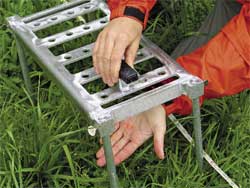
Soil cover is quantified at each quadrat based on readings from a 20 point fixed frame. There are several types of frames that have been developed. The most appropriate frames are 1) light weight and portable, 2) stable, and 3) easy to assess data points on the ground surface. One frame that meets these criteria uses a laser pointer to identify data points. The frame shown in Figure 12.3 has 20 slots to position a laser pointer. During monitoring, the laser pointer is moved to each of the 20 slots. Soil cover attributes are recorded where the laser hits the ground surface. Contact the authors of this report for more information on this frame.
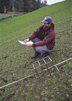
The fixed frame must be located along the tape in a consistent manner throughout the sampling of a unit (Figure 12.2). For instance, the frame might be placed on the right side of the tape with the lower corner of the frame at the predetermined distance on the tape. This procedure would be applied across the entire sampling area. The legs of the frame are positioned so that the surface of the frame is on the same plane as the ground surface (Elliot personal correspondence 2007).
Each data point is characterized from a set of predetermined label descriptors which include, but are not limited to:
- Soil
- Gravel (2mm to 3 inches)
- Rock (> 3 inches)
- Applied mulch
- Live vegetation (grasses, forbs, lichens, mosses)
- Dead vegetation
Ideally, one would quantify only cover in contact with the soil surface. However, differentiating between plant leaves and stems that are in direct contact with the soil as opposed to simply in close proximity to the soil surface can be difficult and not always feasible. In this protocol, the assumption is that if live or dead vegetation is within one inch of the soil surface, it will be recorded as soil cover.
Different levels of vegetative cover will block the view of the soil surface. To circumvent this problem, the quadrat will be clipped of standing vegetation (dead or alive) at a one inch height above the ground surface prior to taking the readings. The clipped vegetation is removed from the plot before the reading is made. This method errs on the side of lower ground cover readings because the standing vegetative material that is clipped and removed would have eventually become ground cover.
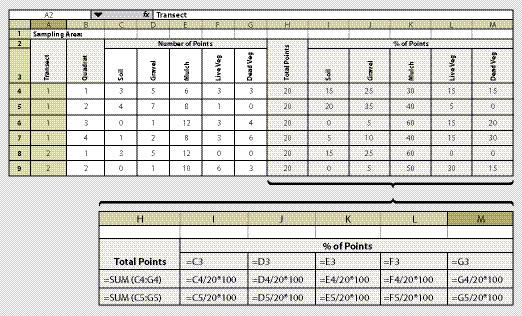
Data can be recorded on a field-going computer or on paper. Recording data on paper bypasses the need for electronic equipment in the field. However, it requires that data be entered into a computer at a later time. The development of a paper form should consider how data will be entered and statistically analyzed. Figure 12.4 shows a spreadsheet for collecting data which also will summarize the data by % of surface in a cover attribute.
12.2.2 Sampling by Digital Camera
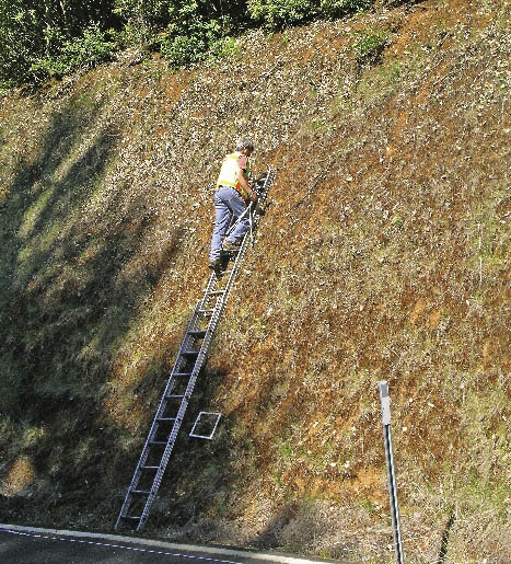
Digital cameras are being used more and more frequently for monitoring plants and animal life. This technology allows the data collector to spend most of the field time laying out transects and taking pictures of quadrats, reducing field time significantly. With recent developments in photo-imaging software, photos can be assessed quickly back in the office. Because these are permanently stored records, digital photographs have several advantages: 1) photographs can be reviewed during the "off" season or "down time," 2) they are historical records that can be referenced years later, and 3) they can be reviewed by supervisors for quality control. In addition, taking digital photographs of ground cover can be accomplished by one person, not two as is often required of fixed frame monitoring. On steeper slopes, using a digital camera to record quadrats is much quicker and simpler than reading attributes from a fixed frame which is often very difficult (Figure 12.6).
Sampling by camera requires the same statistical design and plot layout as the fixed frame method. The difference is that a picture is taken at the quadrat location instead of on-site measurements. In the office, digital photographs are cataloged electronically and a 20-point overlay is placed on the image that identifies the data points to be described (Figure 12.5). The data points are described in the same manner as the fixed frame method.
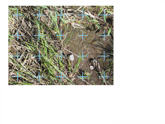
Prior to photo monitoring, the resolution of the images must be determined. Setting the camera at the highest resolution is fine provided the camera has the memory capacity to store large images. It is possible that over a hundred digital images will be recorded for each sampling area. When memory is limiting, it is important to select the minimum resolution that will allow fine surface details to be observed. Resolution should be determined for each camera by taking photos of a soil surface at several camera settings (see the camera manual) and viewing them on a computer screen to determine whether photos are detailed enough for accurate measurement of the soil cover attributes. It is important to have enough memory to store the number of pictures required. Carrying extra memory (as well as an extra battery) is always a good idea.
The camera should be secured to a tripod at a fixed height between 3 to 5 feet above the ground surface. The camera height should be adjusted so it is comfortable for the person sampling while still capable of capturing the image within a photo frame. A photo frame defines the area within which the photograph will be taken. The frame can be easily made from PVC pipe joined together with pipe connectors. There is not a standard frame size however, an 11 in by 14 in frame seems to work well. Prior to each photograph, the transect/quadrat must be recorded within each frame so that each image can be accurately identified later. This can be done with by writing the number on small tags or paper and included in a corner of the frame. Quadrat identifiers are abbreviation of the transect and quadrat numbers (e.g., "4-2" represents the fourth transect/second quadrat).
When the photo frame is in place and the quadrat has been identified, vegetation greater than one inch from the surface of the soil is cut to a height of one inch and removed. The tripod is positioned over the photo frame so the camera is approximately on the same plane as the ground surface. The camera lens should be adjusted so the photo image in the view screen is just inside the quadrat frame. The picture should be taken so shadows from the tripod or the photographer are not in the frame. Cloudy days are often ideal due to the lack of shadows. Clear days, especially when the plots are in direct sunlight, can be difficult because of the extreme shadows. The camera flash can be used under these conditions to reduce the contrasts within the images.
The FHWA and USDA Forest Service have developed a method for evaluating digital photographs by adapting a software program for monitoring underwater coral cover. The program is called "Monitoring soil cover using CPCe digital photo assessment method" and it automates the configuration of a large group of digital photographs so that they are easy to evaluate and record. The program navigates the user to the 20 points on each digitally photographed quadrat at the click of a mouse. At each point the user records the observed soil cover attribute. The data is summarized and can be taken directly into spreadsheets for statistical analysis.
12.3 Species Cover Protocol
The species cover protocol is used to assess the aerial dominance of seeded species. This protocol is used when revegetation standards require that a certain percentage of vegetative cover be composed of native species. For example, revegetation objectives that were agreed upon during the planning phase state that over 50% of the vegetative cover existing on the site two years after construction will be composed of native species that were seeded. Monitoring the vegetative cover through this protocol will assess whether this was accomplished. Since grass and forb cover changes during the season, the timing of species cover monitoring is important. The best time to monitor is during flowering, typically from mid-May through July, because the species are identifiable during this period.
Use of a digital camera is not usually applicable to species cover monitoring because identifying species is not always possible in digital photographs. Sampling is therefore accomplished with a fixed frame. This sampling protocol typically requires a botanist to identify species and another person to help lay out the plots and record data.
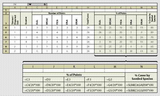
Species cover is quantified at each quadrat based on readings from a 20-point fixed frame (See Section 12.2.1). At each point, the species is recorded on a spreadsheet similar to Figure 12.7. More columns can be inserted on the spreadsheet to account for a larger number of species. The tendency can be to record all species encountered in a sampling area; however, this is not recommended. Instead, we recommend grouping species into such categories as "non-native grasses," or "non-seeded native forbs," which can be useful for later analysis and reporting.
As with all protocols, the sampling design for laying out transects and quadrats depends on the shape of the sampling unit (See Section 12.7), and the number of quadrats to sample depends on the variability of the parameter of interest (See Section 12.8). How the data will be analyzed will be based on the objectives for monitoring (See Section 12.9). These sections should be reviewed before this protocol is used.
12.4 Species Presence Protocol
Determining species cover, as outlined in the previous section, can be time-consuming and expensive. The species presence protocol is an alternative method of determining whether or not species that were seeded are present on the site. While this method still requires a botanist in the field, it takes far less time per plot because only presence or absence of a species is recorded.
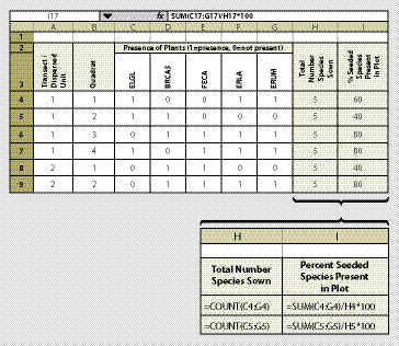
In this method, a fixed frame is placed on the surface of the soil at each quadrat. The size of the fixed frame should be based on what is considered a measurement of success. For instance, for shrub or tree species, having one plant established every 10 ft2 (equivalent to 4,356 plants/acre) would be very successful. However one grass plant every 10 ft2 might not be considered successful. For monitoring most species, we recommend a frame size of 4 ft2 (2 ft on each side) using a PVC pipe with connectors. This size frame is easy to carry and read. Whatever size is used, we recommend that the frame dimension stay the same throughout the monitoring project. Prior to sampling, the species of interest (typically just the seeded species) are identified and recorded on the data form (Figure 12.8). These will be the only species recorded at each quadrat. At each quadrat, the species of interest are evaluated for presence or absence. If the species is present, it is given a "1," and if it is not present, it is given a "0." The data is summarized by the percentage of the species present on the quadrat out of the total number of seeded species.
As with all protocols, the sampling design for laying out transects and quadrats depends on the shape of the sampling unit (See Section 12.7), and the number of quadrats to sample depends on the variability of the parameter of interest (See Section 12.8). How the data will be analyzed will be based on the objectives for monitoring (See Section 12.9). These sections should be reviewed before this protocol is used.
12.5 Plant Density Protocol
Trees and shrubs are typically established from plants (See Section 10.2.6, Nursery Plant Production and Section 10.2.3, Collecting Wild Plants) or cuttings (See Section 10.2.2, Collecting Wild Cuttings and Section 10.2.5, Nursery Cutting Production). Many constructed wetlands are also planted from nursery grown or wild collected seedlings. Monitoring the density of live plants following the first and third year after they are planted is important in order to determine if they have survived and whether the site will need to be replanted. In the case of constructed wetlands, plant density monitoring is conducted to determine whether regulatory requirements were met.
The quadrat in this protocol is a circular plot with a specified radius. We recommend using a 1/100 acre plot, which has an 11.7 ft radius and covers 436 ft2. A staff is placed at plot center and a tape or rope is stretched 11.7 ft. While one person holds the staff, the other walks the circumference of the plot and counts the number of plants within the quadrat. This information is recorded on a spreadsheet similar to Figure 12.9. This spreadsheet reports the number of plants per acre by species. It also summarizes total plants per acre.
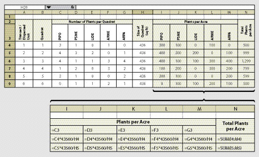
From this spreadsheet plant density can be estimated and an approximate survival rate can be determined by dividing the estimated density (average of column N) by the original planting density (per acre basis from planting records). Plant density monitoring used to determine survival rates are called survival surveys and these are usually conducted in the fall or winter. If the site is planted in the fall or spring and monitoring occurs the following fall, the results are referred to as the "first year survival." Plant density monitoring thereafter, is referred to as the years after planting (e.g., third year sampling is "third year survival").
The sampling design for laying out transects and quadrats depends on the shape of the sampling unit (See Section 12.7), and the number of quadrats to collect from depends on the variability of the parameter of interest as discussed in Section 12.8. (Note that for linear sampling designs, there is only one randomly placed quadrat per transect.) How the data will be analyzed will be based on the objectives for monitoring (See Section 12.9). These sections should be reviewed before this protocol is used.
12.6 Plant Attributes Protocol
The plant attributes protocol is used to measure plant growth. This protocol can be used to assess growth responses between revegetation treatments or revegetation units, and to determine whether standards pertaining to growth requirements were met. Typically only sensitive areas, such as visual corridors or wetlands, have stated growth requirements that must be monitored. This protocol might have limited applicability to most revegetation projects.
Any part of a plant can be measured, and the selection of an attribute is dependent on the species being sampled. Common attributes include:
- Total height — trees and most shrubs
- Last season's leader length — most trees
- Stem diameter — shrubs and trees
- Crown cover — shrubs, forbs, and grasses
- Weight — grasses and forbs
Total height is typically measured from the ground surface to the top of the bud. If the plant has several leaders (or tops), the most dominant leader is used for measurement. Last season's leader growth can be observed in most tree species. For conifers, leader growth is measured from the last whirl of branches to the base of the bud. Comparing leader growth from year to year can indicate whether plants are healthy and actively growing. Stem diameter can be used to measure most trees and shrubs; in this method, the basal portion of the plant is measured with calipers at the ground surface. Crown cover is more conducive to spreading plants, such as shrubs, grasses, and forbs. This measurement requires the use of a large frame with grids or points that can be placed over the plant to obtain an aerial coverage. Weight of the plant is typically used for grasses and forbs. Foliage is clipped at the base and weighed immediately for fresh weight, or dry weight after the sample has been oven-dried.
| Figure 12.10 — A spreadsheet is shown here for recording one species and one attribute. This spreadsheet can be developed to record several attributes or several species. |
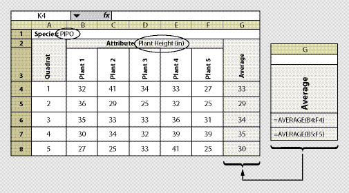 |
Sampling plant attributes should be narrowed to a species of interest. It is probably not necessary to measure all species on a site. Those species that are easy to measure and will dominate the site are the best to sample (typically trees and shrubs). It is not necessary to sample all plants in a quadrat. We suggest a minimum sample of 5 plants from each species. An unbiased way to select which plants of each species to monitor is to sample those plants closest to plot center. If there are not enough plants in the quadrat to sample, then the nearest plants outside of the quadrat should be sampled.
The measurement for each plant is recorded in a data sheet similar to Figure 12.10. The species and the attribute being measured must be identified on each sheet (cell B2). The number of quadrats to establish depends on the variability of the plant attribute which is discussed in Section 12.8. How the data will be analyzed is based on the objectives for monitoring (See Section 12.9). These sections should be reviewed before this protocol is used.
12.7 Sampling Area Design
Three basic sampling designs are used to monitor revegetation units depending on the shape or geometry of the sampling areas. The primary objective of these designs is to provide even spatial coverage of sampling locations within revegetation units that results in unbiased data collection. The three types of designs that will be covered are:
Linear (See Section 12.7.1). Long and narrow sampling areas, such as road cut and fill slopes, are sampled using a systematic series of transects, oriented perpendicular to the road, along which are located a set of quadrats. Each transect is treated as the primary experimental unit for statistical analysis.
Rectilinear (See Section 12.7.2). For more rectilinear sampling areas, a systematic grid (that is, a checkerboard) of quadrats is sampled, and each quadrat is treated as the primary experimental unit for statistical analysis.
Dispersed (See Section 12.7.3). When a series of discrete areas (e.g., planting pockets, planting islands) are encountered, a systematic or grid sample design of dispersed areas is identified for sampling. Depending on the geometry and size of these areas, either complete enumeration (measuring all plants) or subsampling using transects or grids is employed within selected areas.
12.7.1 Linear Sampling Areas
Linear areas, such as cut and fill slopes and abandoned roads, are sampled using a systematic series of equally spaced transects. Each transect has varying numbers of quadrats (plots), depending on the length of the transect. When the revegetation unit is fairly uniform in width, each transect will have approximately an equal number of quadrats; when the width of the revegetation unit is highly variable, there will be unequal numbers of quadrats per transect. In either case, each transect is treated as the primary experimental unit.
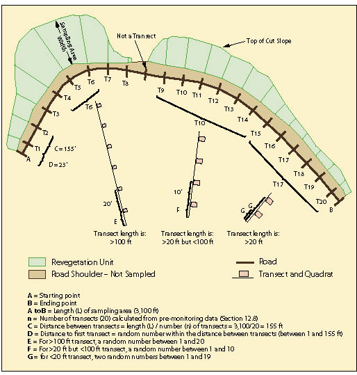
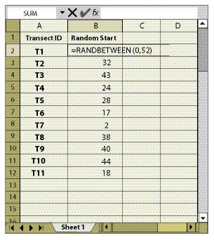
Figure 12.11 shows a typical sampling design for a linear area. In this example, the sampling area included only those portions of the cut slope that were seeded; it did not include road shoulders or ditch line. For statistical analysis, the number of transects (n) to collect was estimated to be 20 based on pre-monitoring data (See Section 12.8). Spacing the 20 transects equally along the sampling area was calculated by dividing the total length of the sampling area by the number of transects to obtain the distance between transects (3,100/20 = 155 ft). Locating the first transect was done in an unbiased way by generating a random number between 1 and 155 using the random number spreadsheet function shown in Figure 12.12.
Transects are laid out by establishing a line perpendicular to the edge of the road. The transect begins at the edge of where seeding or other treatments were completed, which is typically beyond the road shoulder and ditch. Each transect contains a group of evenly spaced quadrats.
The spacing between quadrats vary by the length of the transect:
- <20 ft transect lengths. For sampling areas where transect lengths are less than 20 feet, 2 quadrats are installed. Two random numbers (G) are generated between the numbers 1 and 19. These numbers indicate the location of each transect.
- >20 and <100 ft transect lengths. For sampling areas where transect lengths are between 20 and 100 feet, quadrats are placed at 10 foot intervals. The distance to the first quadrat will be based on a random number between 1 and 10 feet.
- >100 ft transect lengths. These long transects have 20 feet between quadrats. The distance to the first quadrat will be based on a random number between 1 and 20 feet.
For the Plant Density and Plant Attribute protocols, only one quadrat is randomly located within each transect. The location is determined by assigning the RANDBETWEEN random number function to the length of each transect (Figure 12.12).
12.7.2 Rectilinear Sampling Areas
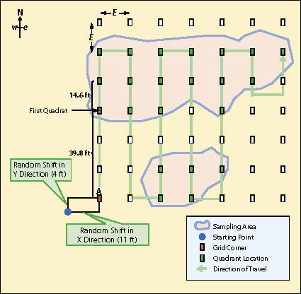
When sampling areas are more elliptical or rectangular in shape, or composed of several large irregular polygons, the sampling design will be based on a rectangular grid of quadrats systematically located with a random starting point. Figure 12.13 shows an example of such a sampling design. Notice that this design is different from the linear sampling design in that there are no transects. The quadrat in this sampling design is the primary experimental unit, not the transect.
To determine the grid spacing (E) for the quadrat locations, the area of the sampling unit must be obtained from maps, and the number of quadrats to be sampled (n) must be determined from pre-monitoring data (See Section 12.8.2). The following equation gives the length of each side of a square grid (E):
![]()
For example, the sampling area in Figure 12.13 covers 4,262 ft2 and it has been determined from pre-monitoring data that approximately 20 quadrats are necessary to attain the statistical sampling requirements for this sampling area. The formula indicates that each side (E) of the grid should be 14.6 ft:
![]()
A starting point of the grid is arbitrarily located in any corner of the study area. To avoid biasing the placement of the quadrats, the corner of the grid must be shifted by assigning random numbers to the x and the y coordinates as shown in Figure 12.13. This is called a systematic design with a random start. It provides equal likelihood that any point in the study area is included in the sample unless there are obvious systematic patterns in the site such as planting rows. In this case, the random number shifts were 11 ft in the horizontal direction and 4 ft in the vertical direction.
In this example, the monitoring team would locate the starting point in the field. Taking a true north bearing, the team would measure 39.8 ft (10.6+14.6+14.6 = 39.8) to take the first plot. They would measure 14.6 ft on that bearing to locate the next quadrat. After they collected data from the last quadrat in that line, they would take a due east bearing and walk 14.6 ft to locate the next plot. This system of sampling would continue until the entire area has been sampled.
12.7.3 Dispersed Area Sampling
When sampling areas occur as small, distinct areas, a two-stage sampling design is recommended. The first stage is to determine which dispersed areas to sample and the second stage is determining how to sample within each selected area. For the first sampling stage we suggest that a minimum of 20 dispersed areas be monitored within each revegetation unit. If there are 20 dispersed areas or fewer, then all dispersed areas would be sampled. If there are more areas than 20, then they must be sampled using one of two sampling designs. For dispersed areas that range in sizes from small to large and are mapped, the systematic sampling design is used (See Section 12.7.3.1). If the dispersed areas are small or are not mapped, then a grid sampling design is used (See Section 12.7.3.2). In most cases, the grid sampling method is recommended.
12.7.3.1 Systematic Sampling of Dispersed Areas
First Stage — The systematic sampling method of dispersed areas assumes that the dispersed areas have been mapped and identified. The dispersed area in this method is the experimental unit. In this approach, the dispersed areas are numbered sequentially by progressing from one dispersed area to the next closest dispersed area. Determining how to calculate the number (n) of dispersed areas to sample is presented in 12.8.3. Odd- or even-numbered dispersed areas are selected based on a random number using the RANDBETWEEN function. For example, if there were 40 dispersed areas (N) but only 20 dispersed areas needed to be sampled (n), then 50% of the dispersed areas would be sampled (n/N). A random number using RANDBETWEEN(1,2) is used. If the function returns a "1" the odd numbered dispersed areas are selected; if 2, then even numbered areas are selected. Figure 12.14 provides a schematic depiction of such a design.
Second Stage — Once the dispersed areas have been selected, the layout of quadrats within each dispersed area is determined. A grid-based sampling design, as described in Section 12.7.2, can be used. To determine the grid spacing (E) for the quadrat locations, determine whether the size of the dispersed area is >1,600 ft2 or <1,600 ft2 (1,600 ft2 is a 40 by 40 ft area). Depending on the sample size, the number of quadrats will be:
- Less than 1,600 ft — 4 quadrats
- Greater than 1,600 ft — 8 quadrats
Using the following equation, the grid sides (E) are determined where n = 4 or 8 depending on the size of the dispersed area and Area is the estimated dispersed area size.

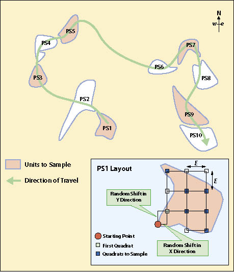
This calculation will be made for each dispersed area. To avoid biasing the placement of quadrats, a predetermined starting point is decided upon (e.g., the northwest corner of each dispersed area). Random x and y coordinates are generated for each dispersed area that are within the predetermined length of the square grid (E). The corner of the grid is placed at this point and oriented north. The location of the first quadrat is x and y coordinates from the starting point as shown in Figure 12.14.
For the plant density and plant attribute protocols, only one quadrat is randomly located within each dispersed sampling area. The location is determined by assigning the RANDBETWEEN random number function to the number of quadrats determined for the dispersed area. The random number that is generated is the quadrat selected for sampling.
12.7.3.2 Grid Sampling of Dispersed Areas
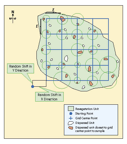
First Stage — A grid sampling design is used on projects where dispersed areas have not been mapped and there are more than 30 areas. This sampling design is typically used on projects where dispersed areas are numerous and the sizes of the areas are small. In this sampling design a grid is placed over the revegetation unit as shown in Figure 12.15 and the dispersed area nearest to the grid center is selected for monitoring. One quadrat is randomly placed in each dispersed area and this becomes the experimental unit.
Determining the grid cell dimensions (E) is accomplished by using the following equation:
where the area is the total area of the revegetation unit and n is the number of quadrats to locate (See Section 12.8.3 for determining number of quadrats to sample).
The grid is laid out unbiasedly by locating a starting point just outside the revegetation unit and assigning random numbers to the x and the y coordinates. The corner of the grid is placed at the x and y offset point and oriented north. In the field the grid centers are located using a compass and measuring tape. At each grid center, the closest dispersed area is selected for monitoring. If there are no dispersed areas found within half the distance between grid centers (E/2), then the monitoring team moves on to the next grid center. For revegetation units that have dispersed areas somewhat clustered, grid centers will sometimes be located where there will be no dispersed areas to sample. For this reason, when calculating the grid cell dimension (E) from the equation above, the number of quadrats (n) should be increased 10 to 20% to compensate for grid centers where dispersed areas are not in close proximity.
Second Stage — For seedling density and seedling attribute protocols, dispersed units that are selected for sampling may be small enough that plant measurements can be exhaustive (e.g., all plants are measured). These situations usually arise when seedlings are planted in planting islands, benches, or pockets. When this is not possible, or other protocols, such as soil cover, species cover, or species presence protocols are being used, one quadrat is located randomly by facing away from the dispersed area and throwing a rock, hammer, or something heavy and selecting the quadrat location where it lands.
12.8 Sample Size Determination
The number of experimental units needed to statistically sample a revegetation area is based on the variability of the attributes being sampled. By pre-sampling representative areas prior to monitoring, an approximate number of quadrats and transects can be determined. Using pre-monitoring data, however, does not always guarantee enough samples will be taken. There will be projects where pre-monitoring data will not predict the variability, and more samples will be needed. This is usually discovered after reviewing the data back at the office. At that time, the monitoring leader has to decide whether to return to the site and collect more data. To avoid this expensive scenario, we recommend that each revegetation unit be composed of at least 20 primary experimental units (20 transects for linear sampling design, 20 quadrats for rectilinear, or 20 dispersed areas for dispersed area sampling design).
Taking a minimum of 20 samples should help prevent the possibility of having to return to the site to collect more data. The cost of collecting a small amount of extra data from quadrats or transects during initial monitoring is typically low relative to the cost of personnel, equipment, and travel to and from the project area. Taking a minimum of 20 samples is considered a prudent precaution. While 20 samples should be enough for most projects, sample size calculations should nevertheless be conducted to determine whether additional primary experimental units may be needed to achieve the precision requirements of the monitoring plan.
Sample size determination methods must be tailored to the monitoring objectives and sampling area design. For compliance objectives for linear area sampling design see Section 12.8.1, rectilinear sampling area design see Section 12.8.2, and dispersed areas see Section 12.8.3. For determining sample size for comparing treatments areas see Section 12.8.4
12.8.1 Comparing Means with Standards — Linear Sample Size Determination
To calculate the minimum sample size for linear sampling areas (See Section 12.7.1), it is necessary to approximate the expected sample mean and the range in values. A visual estimate of the mean and the range of values may be adequate. However, for more precise estimates, 4 transects can be sampled to establish estimates of the mean and range of values. The following is a quick method of determining the number of transects to sample based on pre-monitoring data collection:
- Drive the entire revegetation unit and note the different extremes of revegetation success.
- Find 4 areas that represent the extremes and lay out a transect in each area.
- Randomly place 2 quadrats within each transect to collect data on the attribute of interest (e.g., % ground cover).
- For each transect, average the quadrat values (4 averages).
- Calculate the average of the 4 transect averages and calculate the range (difference between highest and lowest values of the 4 averages).
- Apply the range and the average to the following equation to obtain the minimum number of transects needed to monitor the revegetation unit (equation based on a sample size of 20% of the true population value with 90% confidence).
n = (0.838 * Range)2 / (0.2 * x)2
The number of transects (n) obtained from this quick assessment is used to determine the layout of the monitoring design as discussed in Section 12.7.
Example: Suppose that monitoring is to be conducted along a road cut to determine the percentage of soil cover. The monitoring objective is to estimate mean percent cover to within 20% of the true population value with 90% confidence. Four transects that represent a range in conditions are laid out within the revegetation unit. These transects do not need to be located randomly, but rather should be sited to capture the range of values observed in the sampling area. It is better to over-estimate the range of values, as this will tend to result in a conservative estimate of the sample size. The data set and equation is shown in Figure 12.16.
Using the equation presented above, an estimated 13 transects were calculated for a minimum sample size. Although the minimum sample size is estimated at 13, it is still recommended that at least 20 transects be sampled because the cost of additional transects (should the actual monitoring data be more variable than the pre-monitoring data) is minor relative to the expense of returning to the site and collecting more data.
12.8.2 Comparing Means with Standards —Rectilinear Sample Size Determination
When a grid of quadrats is to be implemented (See Section 12.7.2), the sample size calculations use quadrat measurements as opposed to the transect averages that were used in linear sampling areas. The steps involved in calculating the number (n) of quadrats are:
- Visit the entire revegetation unit and notice the different extremes of revegetation success.
- Find 4 areas that represent these extremes and lay out a transect in each area.
- Randomly place 2 to 3 quadrats within each transect to collect data on the variable of interest (e.g., % ground cover).
- Average the quadrat values (8 quadrat values to average)
- Calculate the range of all 8 samples (difference between highest and lowest values).
- Apply the range and the average to the following equation to obtain the minimum number (n) of transects needed to monitor the revegetation unit.
n = (0.838 * Range)2 / (0.2 * x)2
| Figure 12.16 — Example of how to calculate the number of transects needed to be established from pre-monitoring data set. | 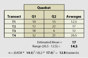 |
Using the data from the previous example (Figure 12.16), the 8 quadrats would be averaged. While the mean in this example would still remain at 17, the range has spread to 26 (maximum 32 minus the minimum 6) The number of quadrats to sample would be 41:
n = (0.838 * 26)2 / (0.2 * 17.0)2 = 41.1
12.8.3 Comparing Means with Standards — Dispersed Area Sample Size Determination
Systematic Sampling Method: The systematic sampling method is used when the dispersed areas are mapped. The experimental unit in this design is the dispersed area.
- Find 4 dispersed areas that represent the extremes of the attribute of interest and lay out.
- Randomly place 2 quadrats within each dispersed area to collect data on the attribute of interest (e.g., % ground cover).
- For each dispersed area, calculate the average of the 4 dispersed areas' averages and the range.
- Apply the range and the average to the following equation to obtain the minimum number of dispersed areas needed to monitor in a revegetation unit (equation based on a sample size of 20% of the true population value with 90% confidence).
n = (0.838 * Range)2 / (0.2 * x)2
Grid Sampling Method: The grid sampling method is used for revegetation units that have small dispersed areas that have not been mapped (See Section 12.7.3.2). Since only one quadrat is located in a dispersed area, the quadrat becomes the experimental unit. The number of quadrats to sample is estimated by following these steps:
- Visit a range of dispersed areas and select 4 dispersed areas that represent these extremes of site conditions.
- Randomly place 1 quadrat in each of the 4 dispersed areas and collect data on the parameter of interest (e.g., % ground cover).
- Calculate the average and range in values.
- Apply the range and the average to the following equation to obtain the minimum number (n) of dispersed areas to sample.
n = (0.838 * Range)2 / (0.2 * x)2
12.8.4 Sample Size for Comparing Means Among Treatment Groups
When determining the sample size for comparing treatment differences (See Section 12.9.2), it is not necessary to differentiate between linear, rectilinear, or dispersed sampling designs. Sample size determinations can be made by following these steps:
- Review each treatment area to be compared. These can be different revegetation units or different types of revegetation treatments.
- From each treatment area, collect data from 2 transects composed of 2 quadrats. These should represent a range of extremes for a total of 4 transects.
- Determine the range.
- Determine delta. Delta defines the level of significance that is needed for monitoring, or the meaningful difference in measurement output. For example, calculating bare soil at 1% differences in means would be unimportant, that is, the difference between 8% and 9% bare soil is too fine a distinction to make. A 5% difference might be important if the amount of data that is needed to be collected was not great. More than likely, a 10% difference (e.g., the difference between 10% and 20% bare soil) would be an acceptable delta value for bare soil cover. It is important to note, the smaller the delta value, the more samples need to be collected.
The number of transects (n) can be calculated using a simplified equation:
n = 15.68 / (Δ * 2.059 / Range)2
The number of transects determined from these calculations are applied equally to the two (or more) areas being compared. This equation assumes that tests will be conducted at the delta level of significance and that there will be a difference detected at or greater than an 80% probability. Readers who prefer to apply different assumptions are encouraged to read the backup document to this guide (Kern 2007).
Example: Suppose you are interested in finding out whether a commercial product actually increases plant cover by at least 10% after the first year as advertised. You have set up similar areas, one where the product was applied and one where it was not. A year later, you want to determine whether there is a difference in the percentage of vegetative ground cover. To determine the number of transects to install in each area, you set out 4 transects, 2 in each area. From this information, you find a range in % vegetative ground cover values of 22. You assume that tests will be conducted at the delta level of significance of 10% (important to be able to detect a difference in 10% cover with at least 80% probability). Using the simplified equation stated above, the following number of transects are required for each treatment area:
n = 15.68 / (10* 2.059 / 22)2 = 17.9 transects
In general, using the simple equation provided here, and possibly adding 10% to 20% additional samples as a level of conservatism, is a reasonable approach.
12.9 Statistical Analysis Using Confidence Intervals
This section provides statistical methods for analyzing data collected for all monitoring protocols covered in this chapter. There are three types of analysis based on these monitoring objectives:
- Compliance — determine whether standards were met (See Section 12.9.1).
- Treatment differences — determine whether there is a difference between treatments or changes between years (See Section 12.9.2).
- Trends — determine the degree of vegetation or soil cover change over time (See Section 12.9.3).
The analysis for these objectives uses the concept of confidence intervals for determining the statistical significance of the monitoring data set.
12.9.1 Determine Standards Compliance
The objective behind most monitoring is to answer the following questions: were regulatory standards met? Did we actually do what we stated we were going to do in our reports and commitments to the community in terms of protecting soil and reestablishing native vegetation?
To answer these questions requires comparing the means of the attribute data collected (e.g., bare soil, species presence) with the set standard or stated threshold. For example, a project has a standard of at least 70% soil cover on a road cut near a live stream one year after road construction. Using the soil cover protocol, data is collected on 20 transects and a mean of 81% soil cover is determined by averaging the quadrat means. At this point, the reader might conclude that the standards were met. From a statistician's point of view however, the data displayed in this context is inconclusive because we do not know, or cannot account for, the variability of the soil cover in the sampling area. In other words, how do we know how good the number is? Is it really depicting what is happening on the site? If another person were to use the soil cover protocol in the same sampling area, but at a different spot, would the soil cover be exactly 81%? This is highly unlikely because of the high variability of soil cover.
Confidence intervals give us the means of predicting, at a chosen level of certainty, that the soil cover value collected anywhere in the sampling area will be within a stated range. Confidence intervals are an alternative to saying, "We think the soil cover at any point in the sampling area will be around 81%." Using confidence intervals we can say instead that, "we are 90% confident that if the study were repeated at this site 10 times, 9 out of 10 times the average soil cover estimate would be within our confidence limits." If you want to feel more confident than that about your predictions (most scientists working in the health fields want to be very certain) you might decide you want to have confidence intervals based on 95% or even 99% certainty. If this is the case, the confidence interval would be much wider.
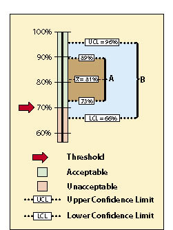
The data sets from very different revegetation units are shown in Figure 12.17 to convey the concept of confidence intervals. While both data sets have the same mean of 81% soil cover, the confidence intervals are very different. Data set A was taken at a site with very uniform soil cover, while data set B had much more variability. For both data sets, we want to define the confidence intervals at a 90% confidence. Notice that the confidence interval for data set B is much wider than data set A since it has greater variability.
With confidence intervals, we can say with greater certainty whether the standard of 70% soil cover was met or not. We can state with 90% confidence that data set A met the standards because the lower confidence limit (73%) is above the stated standard of 70%. Data set B, on the other hand, poses some problems. We cannot say with 90% confidence that the unit average is above the standard of 70%. The lower confidence limit of data set B is 66%, or 4% below the standard. The reader might argue that, because the mean is above the standard, the standards were met ("hey, it's close enough!"). To statisticians, however, the fact that the lower confidence interval is below the stated standards indicates a fair amount of uncertainty. They would tell you that you cannot make that statement without getting more data or changing how confident you are with the prediction.
One of the main purposes for monitoring roadside vegetation is to document successful project completion. Statistically based sampling designs and analysis provides an objective way to describe revegetation performance. An understanding of confidence limits and their interpretation is critical to documenting that standards have been met. The following section outlines how confidence intervals are calculated and compared with standards. It is organized by sampling design: linear, rectilinear, and dispersed.
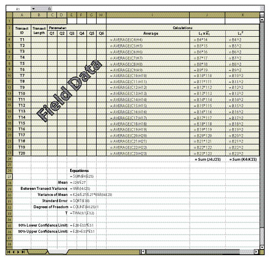
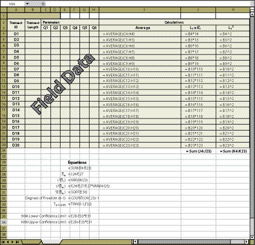
| Figure 12.18 — Confidence intervals for linear sampling designs can be easily obtained by copying equations and format of this spreadsheet. |
 |
12.9.1.1 Calculating Confidence Intervals for Linear Sampling Design
Figures 12.18 and 12.19 give examples of how to calculate confidence intervals from a data set for a linear sampling area (See Section 12.7.1). Figure 12.18 shows how to set up the spreadsheet and Figure 12.19 shows what a typical data set might look like. Once you have set the spreadsheet up exactly as it is shown in Figure 12.18, it needs to be tested by entering the data shown in Figure 12.19. If the confidence intervals in your spreadsheet do not match those of Figure 12.19, then you will need to review the spreadsheet for errors in copying. Make sure that the equations are in the same cells as shown in Figure 12.18. To obtain a number for "T" (cell E31) the Excel ToolPak must be installed. To do this, go to the toolbar and select Tools, Add-Ins, and check the box next to Analysis ToolPak.
The essential data needed to complete the spreadsheet in Figure 12.18 is:
Transect Length (Column B) — This is the total length of the transect recorded in the field at the time the transect is laid out.
Parameters (Cell C2) — There may be several parameters collected at each quadrat. The parameter (or attribute) to be evaluated should be stated at the top of the quadrat columns. For instance, in Figure 12.19, the attribute to be analyzed is "% bare soil," which was obtained using the Soil Cover Protocol spreadsheet (Figure 12.4). Only one attribute can be measured on a spreadsheet. Gravel, rock, live and dead vegetation, for instance, are often collected in the soil cover protocol. If a statistical analysis of these attributes is needed, a spreadsheet must be developed for each attribute. While not all attributes need to be statistically analyzed, it is important to analyze those attributes that have been identified for measurements of success (e.g., % bare soil or % soil cover).
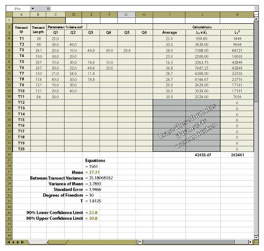
| Figure 12.19 — The spreadsheet developed from Figure 12.18 can be checked for accuracy by entering the data in this spreadsheet. |
 |
Field Data (Columns C Through H) — The data collected at each transect and quadrat for the parameter of interest is typed into these cells. This information comes from the spreadsheets developed for each protocol (Soil Cover Protocol — Figure 12.4, Species Cover Protocol — Figure 12.7, Species Presence Protocol — Figure 12.8, Plant Density Protocol — Figure 12.9, and Plant Attributes Protocol — Figure 12.20) and it is entered and summarized by transect.
Columns I and J — If fewer than 20 transects were taken, the equations in the cells of column I and J that do not have data must be cleared for the spreadsheet to work (see highlighted cells in Figure 12.19).
12.9.1.2 Calculating Confidence Intervals for Rectilinear Sampling Designs
Figure 12.20 shows how to calculate confidence intervals for rectilinear sampling areas (See Section 12.7.2). Copy the equations exactly as they are shown in Figure 12.20 into your spreadsheet. Once you have created the spreadsheet, check the confidence limits in your spreadsheet. They should match those shown Figure 12.20. If they do not, then review your spreadsheet for errors. To obtain a number for "T" (cell C28) the Excel ToolPak must be installed. To do this, go to the toolbar and select Tools, Add-Ins, and check the box next to Analysis ToolPak.
The essential data needed to complete the spreadsheet is:
Parameters (Cell C2) — The parameter to be evaluated should be stated at the top of the quadrat columns. In this example, total cover for "seeded" native species was obtained from Figure 12.7, but any number of site attributes can be analyzed. Copying column C and pasting it in the columns to the right allows for multiple attributes to be analyzed in one spreadsheet.
| Figure 12.20 — This figure shows how confidence intervals are obtained from a spreadsheet developed for rectilinear sampling designs. |
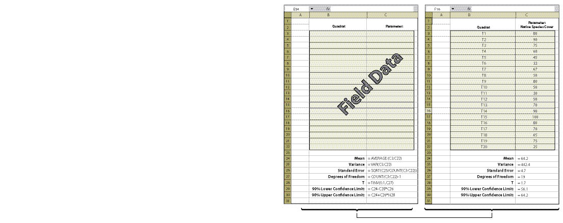 |
Field Data (Columns C Through H) — The data collected at each quadrat for the parameter of interest is typed into these cells. This information comes from the spreadsheets developed for each protocol (Soil Cover Protocol — Figure 12.4, Species Cover Protocol — Figure 12.7, Species Presence Protocol — Figure 12.8, Plant Density Protocol — Figure 12.9, and Plant Attributes Protocol — Figure 12.10).
12.9.1.3 Calculating Confidence Intervals for Dispersed Sampling Design
There are two methods for determining confidence intervals for dispersed sampling design — the systematic sampling design (See Section 12.7.3.1) and the grid sampling design (See Section 12.7.3.2). Confidence intervals for the grid sampling design are obtained by using the spreadsheet shown in Figure 12.20. For the systematic sampling design, Figure 12.21 is used. The essential data needed to complete the spreadsheet is:
Dispersed Area ID — For some projects, not all dispersed areas will be sampled. Identify in Column A which areas were sampled.
Number of Quadrats (Column B) — Specify the number of quadrats that were sampled for each dispersed area.
Parameters (Cell C2) — There may be several parameters collected at each quadrat. The parameter to be evaluated should be stated at the top of the quadrat columns. Only one attribute can be analyzed on a spreadsheet. Gravel, rock, live and dead vegetation, for instance, are often collected in the soil cover protocol. If a statistical analysis of these attributes is needed, a spreadsheet must be developed for each attribute. While not all attributes need to be statistically analyzed, it is important to analyze those attributes that have been identified for measurements of success (e.g., % bare soil or % soil cover).
Field Data (Columns C Through H) — The data collected at quadrats for each dispersed area for the parameter of interest is typed into these cells. This information comes from the spreadsheets developed for each protocol (Soil Cover Protocol — Figure 12.4, Species Cover Protocol — Figure 12.7, Species Presence Protocol — Figure 12.8, Plant Density Protocol — Figure 12.9, and Plant Attributes Protocol — Figure 12.10) and it is entered and summarized by dispersed area.
| Figure 12.21 — Confidence intervals for dispersed areas using the systematic sampling design can be obtained by using the equations shown in this spreadsheet. |
 |
Columns I and J — If fewer than 20 dispersed areas were taken, the equations in the cells of column I and J that do not have data must be cleared for the spreadsheet to work (see highlighted cells in Figure 12.19).
12.9.1.4 Interpreting Confidence Intervals for Compliance
Confidence intervals, as stated previously, are used to evaluate the success of a revegetation project relative to specified standards or stated goals. Suppose that one of the objectives of the revegetation plan was to establish at least 65% total cover over the soil to protect against surface erosion. Or stated another way, the objective is no more than 35% bare soil exposed one year after revegetation treatments were applied. In the example shown in Figure 12.19 (cells E34 and E35), the confidence interval was below 35%. We can say with 90% level of confidence that the objectives were met. But what if the confidence interval was either above the standard or straddled the standard?
Figure 12.22 shows four possible scenarios for confidence intervals that the revegetation specialist may encounter. Scenario A is a case where the data supports the conclusion at 90% confidence that the project met the standard. Scenario B did not meet the standard because the lower confidence limit was above 35% bare soil.
Scenario C is a case where the mean meets the standard, but the upper confidence limit is above the standard. It cannot be said with 90% confidence that the standards were met. At this point you might ask how important it is to know whether the standards were met or not. If the site directly influences a live stream, it might be very important to know. However, if streams are miles away, it might suffice to report that the there was some uncertainty whether the standards were met. If you determine that you need to be more certain about the results, more data will need to be collected.
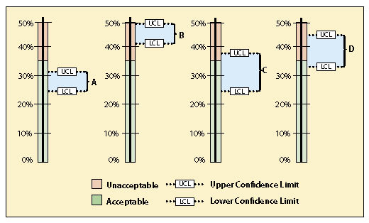
Scenario D is a case where the mean does not meet the standard, but the lower confidence limit is below the standard of 35% bare soil. One might state that this project did not meet the standards, but this still could not be stated with 90% confidence. In this scenario, more transects could be taken to narrow the confidence interval and hope that the results do not straddle the standard. Another option might be to take measures that would decrease the amount of bare soil to meet the standards. This could include more seeding or mulch application. A resampling of the site later would reveal whether the standards were met.
12.9.2 Determine Treatment Differences
There will be opportunities to compare the effects of different revegetation products or methods on plant establishment and growth using monitoring data. Some of these opportunities will be planned (e.g., trying a new product), and some will be mistakes (e.g., inadvertently doubling the rate of mulch). Planned or unplanned, when different revegetation activities have occurred within a revegetation unit, monitoring can be designed to assess whether there is a different vegetative response between those activities or treatments. Note: The monitoring design outlined in this section will not replace a well-designed study or experiment; we suggest that if more conclusive results of treatment differences are required, a study should be designed with statistical oversight.
The confidence interval concept is applied in this section to determine differences between new revegetation treatments (new treatments) and routine revegetation methods (standard treatments). Three possible outcomes are possible when new treatments are compared to standard methods: 1) the new treatment results in a favorable increase in the measured parameters over the standard treatment (positive difference), 2) the new treatment results in a decrease (negative difference), or 3) there is no positive or negative difference (no difference). Using confidence intervals, it is possible to determine which of these outcomes is statistically supported for any monitoring data set. In this method, the means and variance of means are calculated for both the new treatment and standard treatment and a confidence interval is calculated for the certainty of the treatment differences.
The following example demonstrates how a confidence interval is determined and how it can be used to interpret two data sets. During a hydroseeding operation, someone discovers that the rate of fertilizer application was mistakenly applied at twice the normal rate in one area. This area was staked in the field and visited by the project team a year later. Some on the team believed that there was more vegetative ground cover where fertilizer was doubled; others felt that there was actually less. One or two on the team did not believe they could make either call. Since monitoring was going to take place a few weeks later, they decided to design a monitoring protocol to answer the question, "Was there a positive, negative, or no response of vegetative ground cover to the application of additional fertilizer?"
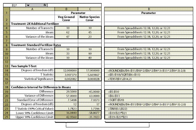
Within the framework of monitoring that was already scheduled for this revegetation unit, a monitoring strategy was developed. The soil cover protocol was used (See Section 12.2) along with the linear sampling design since this was a road cut (See Section 12.7.1). Each treatment area was considered a separate sampling unit, and monitoring took place independently of each other. The data from each treatment area was summarized from Figure 12.4 into % vegetative ground cover and entered into Figure 12.18 to obtain means and variance of means. Number of transects, means, and variance of means for each treatment were then entered into Figure 12.23 (cells B4—B6 for the new treatment and B9-B11 for the standard treatment), producing a confidence interval (cells B24 and B25) for comparison.
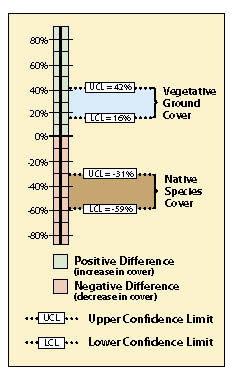
The results of this analysis showed that the standard rates of fertilizer had an average vegetative ground cover of 33% (cell B10) as compared to 62% (B5) for double the fertilizer rate. While this looks like an obvious difference, how certain could the team be? A confidence interval was derived to answer that question. In this example, the confidence interval (at 90% confidence) showed that additional fertilizer significantly increased vegetative ground cover. This can be shown graphically in Figure 12.24. The 2X fertilizer treatment increased ground cover a minimum of 16% over the standard treatment (lower confidence limit) to as high as 42% ground cover (upper confidence limit).
The team accepted these results and commented that they should increase fertilizer rates for future projects. One member posed the question, "We might have achieved better cover on this site during the first year, but is it the vegetative cover we really want?" Since the monitoring team was still on the project site, they resampled the two areas using the species cover protocol (See Section 12.3). In this protocol, native and non-native annuals and perennials were recorded at each quadrat. Confidence intervals were determined for each treatment for native perennial cover (Figure 12.23, cells C24 and C25). They learned, in this case, that additional fertilizer had a negative effect on the establishment of native perennial cover (Figure 12.24). But what if the upper confidence interval in this example had been positive and the lower confidence interval had been negative? In this case, it would have to be concluded that there was no difference between treatments at 90% confidence.
12.9.3 Determine Trends
The last of the three objectives for roadside monitoring is assessing trend, or the degree of vegetative or soil cover over time. The reason to perform this type of monitoring is usually based on the need to understand how growth patterns of certain species or soil cover changes over the years. Many monitoring protocols employ permanent monitoring plots or transects that can be repeatedly and accurately revisited for sampling. We take the approach that collecting data in the same location over time is not feasible for roadside monitoring because of the hazards to road maintenance personnel and to the public of placing permanent stakes in road corridors. In addition, permanent markers are often hard to relocate years later or can move due to the instability of steep cut and fill slopes. In this section we offer a statistical analysis that does not require locating and resurveying of exact quadrats.
The confidence interval concept is applied in this section to determine if there are differences in attributes from one sampling date to another. Three outcomes are possible when comparing data from one sampling date to the next: 1) plant or soil cover attributes have increased since the last sampling period (positive difference); 2) ) plant or soil cover attributes have decreased since the last sampling period (negative difference); or 3) either there was no change in plant or soil cover attributes or the number of samples was inadequate to detect the amount of change that occurred. Using confidence intervals it is possible to make statistically valid statements regarding the observed outcomes.
The following example demonstrates how a confidence interval is determined and how it is used to interpret data taken at different sampling dates. Members of the revegetation team believed that California brome (Bromus carinatus) was a short lived species; that it established well after seeding but by the fifth year it had very little presence on most sites. They also believed that Idaho fescue started out slowly but gained dominance over time. The team felt that by understanding these trends they might develop a better seed mix for sites similar to the ones they were monitoring. The question they posed was: "is there a positive, negative, or no difference in the cover of California brome and Idaho fescue from the first year to the fifth year after seeding?"
This question required the use of the species cover protocol (See Section 12.3) since dominance was being expressed as % crown cover for each species. Linear Sampling Design was used for both monitoring dates because the sampling area was a long cut slope. The data from each sampling date was summarized into % cover for California brome (BRCA5) and entered into Figure 12.18 to obtain means and variance of means. Number of transects, means, and variance of means for each treatment were then entered into Figure 12.25 (cells B9—B11 for earliest sampling date and B4 through B6 for latest sampling date), producing a confidence interval (cells B24 and B25) for comparison. Data entry was also done in the same manner for Idaho fescue (FEID).
The results of this analysis showed that California brome had an average crown cover of 35% (B10) in 2001 but decreased to 27% (B5) in 2006, five years later. Was this a statistically significantly difference? Using confidence intervals, they found that the means were not statistically different at 90% confidence. This can be shown graphically in Figure 12.26. The BRCA5 in 2006 had a maximum of 3% crown cover increase over 2001 and a minimum of -19% ground cover over 2001. Because the upper confidence limit (UCL) was positive and the lower confidence limit (LCL) was negative, the observed data was not adequate to demonstrate a change in % crown cover of California brome with 90% level of confidence.
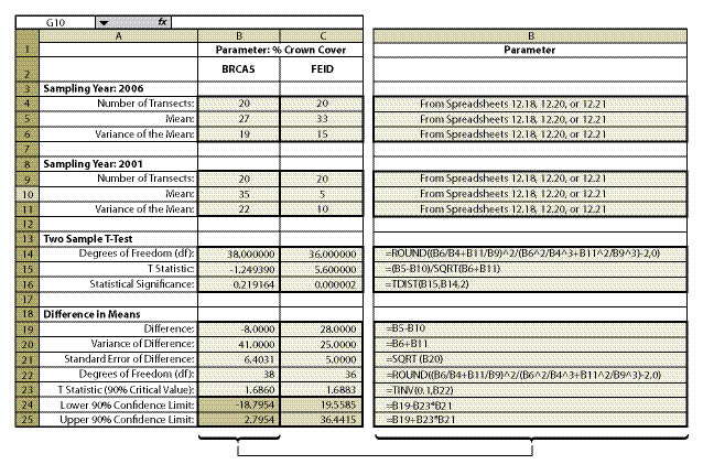
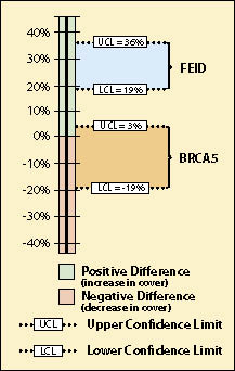
Idaho fescue, on the other hand, did show an increase in mean cover from 2001 to 2006, from 5% (cell B10)to 33% (cell B5) respectively. The team could be 90% confident that the true percent crown cover did indeed increase from 5% in 2001 to 33% in 2006 because the upper confidence limit (UCL) and the lower confidence limit (LCL) were positive (Figure 12.26).
12.10 Summary
This chapter guided the revegetation specialist through a series of steps for collecting field data, developing a sampling design, and statistically analyzing data needed to monitor vegetation on roadsides. Monitoring completes the project cycle by answering the question: Did we accomplish what we proposed in the revegetation plan?
Note: This chapter uses abbreviated scientific names, or plant symbols, from the PLANTS Database
(http://www.plants.usda.gov/java/) to conserve space in spreadsheets. The PLANTS Database includes scientific names, plant symbols, common names, distributional data, images, and species characteristics for vascular plants of the United States.