ROADSIDE REVEGETATION
An Integrated Approach to Establishing Native Plants and Pollinator Habitat

6.3 Plant and Soil Monitoring Procedures
This section describes how to develop and implement a set of statistically based monitoring procedures specific to the revegetation project. It outlines methods to record, summarize, and analyze data. Monitoring personnel can obtain Excel® workbooks, which include field data forms and analysis spreadsheets for each procedure, from the Native Revegetation Resource Library. To obtain a list of Excel monitoring procedure workbooks referenced in this chapter, type "xls" in the Search field.
The following three questions are answered to develop a procedure for soil and plant monitoring for each sampling unit:
- What is the shape of the sampling unit?
- What are the monitoring objectives?
- What is being monitored?
The answer to these questions will lead the designer to draw from different sections of this chapter. Take, for example, a road cut that is being monitored to determine if soil cover targets conformed to the Storm Water Pollution Protection Plan. Using Figure 6-2, the Linear sampling area procedure would be used because the road cut is long and narrow. Since the objective is to determine if soil cover targets were met, the Compliance and the Soil Cover procedures would be used.
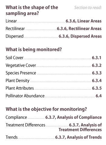
Figure 6-2 | Quick guide to high intensity monitoring procedures
For statistically based monitoring of plant and soil attributes, select a procedure that best answers each of these questions.
Sampling Unit Shape
The shape of the sampling area is important for determining how transects and quadrats are laid out in a sampling unit. For roadside monitoring, there are three main shape categories to choose from, each with a corresponding procedure:
- Linear—This shape is long and narrow and is used to monitor cut slopes, fill slopes, and abandoned roads (Section 6.3.6, see Linear Areas)
- Rectilinear—These sampling areas are typical of staging areas, material stock piles, or large wide areas associated with road construction (Section 6.3.6, see Rectilinear Areas)
- Dispersed—A series of discrete areas that include planting islands and planting pockets (Section 6.3.6, see Dispersed Areas)
Parameters to be Monitored
Parameters for monitoring revegetation projects may include the following, depending on monitoring objectives:
- Soil cover—The amount of exposed bare ground is used to determine if treatments produced adequate soil cover for erosion control (Section 6.3.1)
- Species cover—Used to determine the percentage of aerial or basal cover occupied by individuals or groups of species to quantify species prominence (Section 6.3.2)
- Species presence—Used to assess what species are on the site, how well species in a seed mix became established, or whether noxious, invasive, or undesirable species are present (Section 6.3.3)
- Plant density—Used to assess how many seedlings or cuttings became established after outplanting or how much mortality has occurred (Section 6.3.4)
- Plant attributes—Used to determine growth rates of outplanted seedlings or cuttings (Section 6.3.5)
- Pollinator abundance—Used to assess quantities of honey bees, native bees, and other pollinators (Section 6.4)
Monitoring Objectives
Monitoring objectives also guide how data are collected and statistically analyzed. Procedures have been developed for three basic types of monitoring objectives (Section 6.3.7):
- Compliance—This is often the main purpose for monitoring. It is used to determine if project objectives were met or simply to summarize monitoring data
- Treatment differences—This monitoring objective examines the differences between revegetation treatments or revegetation areas. It is useful to evaluate the effects of different revegetation treatments (seed mixes, fertilizers, soil amendments etc.) on plant establishment
- Trends—This objective evaluates changes in the revegetated plant community in the disturbed area over time. It is used when it is important to understand how plant communities evolve and change
6.3.1 Soil Cover
Reestablishing a soil cover on disturbed sites is important for erosion control. The following soil cover procedures can be used to determine the amount and type of cover existing on the soil surface after slopes have been constructed. The quadrat is the unit of area monitored for soil cover. Exact measurements are based on recording the surface soil condition at data points within each quadrat. Quadrats can be read in the field using a fixed frame or read later in the office from digital photographs of the quadrat taken in the field.
Sampling Soil Cover Using a Fixed Frame
Soil cover is quantified at each quadrat based on readings from a 20-point fixed frame. This method is a point intercept method of estimating cover in a defined area (quadrat). Several types of frames have been developed. The most useful frames are lightweight, portable, and stable. One frame that meets these criteria uses a laser pointer to identify data points. The frame shown in Figure 6-3 has 20 slots to position a laser pointer. During monitoring, the laser pointer is moved to each of the 20 slots. Soil cover attributes are recorded where the laser hits the ground surface.
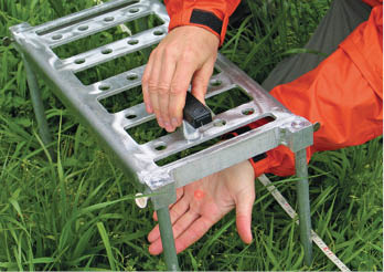
Figure 6-3 | Fixed frame for transect sampling
A fixed frame can be adapted to allow for the positioning of a laser pointer at 20 points in the frame. Soil cover or plant cover attributes are recorded at each laser point. The frame in this example is 8 inches by 20 inches, with 2-inch spacing within rows and 4-inch spacing between rows. The laser is a Class IIIa red laser diode module that produces a 1-mm dot.
Photo credit: David Steinfeld
The fixed frame is located along the tape in a consistent manner throughout the sampling of a unit (Figure 6-4). For example, the frame might be placed on the right side of the tape with the lower corner of the frame at the predetermined distance on the tape. This procedure would be applied consistently across the entire sampling unit. The legs of the frame are positioned so that the surface of the frame is on the same plane as the ground surface.
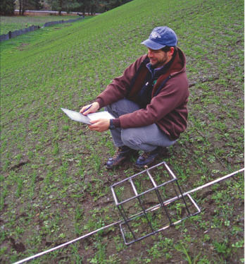
Figure 6-4 | Fixed frame for measuring soil cover
A fixed frame for measuring soil cover is placed at predetermined distances on a transect.
Photo credit: David Steinfeld
Each data point is characterized from a set of predetermined label descriptors that include, but are not limited to, the following:
- Soil
- Gravel (2 mm to 3 inches)
- Rock (> 3 inches)
- Applied mulch
- Live vegetation (grasses, forbs, lichens, mosses)
- Dead vegetation
Ideally, only cover in contact with the soil surface is considered effective ground cover for erosion control purposes; however, differentiating between plant leaves and stems that are in direct contact with the soil as opposed to simply in close proximity to the soil surface can be difficult and is not always feasible. In this procedure, the assumption is that if live or dead vegetation is within 1 inch of the soil surface, it is recorded as soil cover.
Vegetation often blocks the view of the soil surface and is therefore removed prior to data collection. When this is the case, the quadrat is clipped of standing vegetation (dead or alive) at a 1-inch height above the ground surface prior to taking the readings. The clipped vegetation is removed from the plot before the reading is made.
Data can be recorded on a field computer or field recording sheets. Field recording sheets bypass the need for electronic equipment in the field; however, data is entered into a spreadsheet at a later time for analysis. An Excel workbook with field entered forms and a data analysis package (see Figure 6-5) is available for this procedure here.
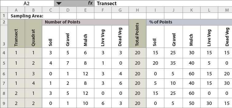
Figure 6-5 | Data collection forms and statistical packages are available on the Native Revegetation Resource Library
A data collection sheet and summary form spreadsheets, such as this one for soil cover, can be downloaded from the Native Revegetation Resource Library by typing in "xls" into the search field and selecting the appropriate workbook. Each section in this chapter has corresponding spreadsheets with instructions, field forms, and statistical packages.
For the Designer
Find this and many other fillable spreadsheets in the Native Revegetation Resource Library by typing "xls" into the search field.
Sampling Soil Cover using Digital Photographs and the Cover Monitoring Assistant (CMA) Program
Digital cameras are being used more frequently for monitoring plants and animal life. This technology allows the data recorder to spend most of the field time laying out transects and taking photographs of quadrats rather than collecting data, thereby reducing field time significantly. With recent developments in photo-imaging software, photographs can be assessed quickly in the office. Because these are permanently stored records, digital photographs have several advantages: photographs can be reviewed during the "off" season or "down time"; they are historical records that can be referenced years later; and they can be reviewed by supervisors for quality control. In addition, taking digital photographs of ground cover can be accomplished by one person, not two as is often used for fixed-frame monitoring. On steeper slopes, taking photographs to record quadrats is quicker and easier than reading attributes from a fixed frame.
Sampling by camera entails the same statistical design and plot layout as the fixed-frame method. The photograph is taken within a quadrat frame with 11-inch by 14-inch dimensions, covering approximately 1 square foot. In the office, digital photographs are catalogued electronically and a 20-point overlay is placed on the image that identifies the data points to be described (Figure 6-6). The data points are described in the same manner as for the fixed-frame method.
The Federal Highway Administration and the U.S. Forest Service have developed a computer program to evaluate digital photographs called Cover Monitoring Assistant (CMA). This program configures each digital photograph taken at a quadrat so it is easy to evaluate in the office. It randomly places 20 points on the photograph and navigates the user to each point where the soil cover attribute is recorded. The data for each photograph is summarized in spreadsheets for statistical analysis. The CMA program has reduced field time and increased data quality significantly. The CMA program information and the User's Guide are available in the Native Revegetation Resource Library.
6.3.2 Species Cover
The species cover procedure is used to assess the above-ground abundance of plant species. This method is a point intercept method of estimating cover in a defined area (quadrat). This procedure can be used when DFC targets state that a certain percentage of vegetative cover be composed of native species. For example, a DFC target from the revegetation plan states that over 50 percent of the vegetative cover existing on the site two years after construction will be composed of native forb species for pollinator habitat and that this cover will consist of species that were in the seed mix. Monitoring vegetative cover with this procedure will determine whether this goal was achieved.
Another advantage of evaluating species cover is the elucidation of patterns of co-occurrences. Weedy species can occur in isolated patches, but often co-occur with other weeds and even among native species. Understanding these distributional patterns and the density of the species assemblages, as they change and develop with the project site, can help the designer select the most effective treatment methods, reduce redundant treatment costs, and prevent damage to the existing native plant community.
Because grass and forb cover changes during the growing season, the timing of species cover monitoring is important. It is ideal to monitor when most plants are flowering, typically mid-May through July for the western United States and July through August for the upper mid-western and eastern states. Bloom periods for forb species also coincide with the optimum period for monitoring pollinator species, so monitoring for species cover and pollinators can be done during the same field visit (Section 6.4).
This sampling procedure typically benefits from a botanists' knowledge to identify species and another person to help lay out the plots and record data. Sampling can be done either with a fixed frame or digital photographs using the CMA program.
Sampling Species Cover Using a Fixed Frame
Using the fixed frame discussed in Section 6.3.1, 20 points are identified in the quadrat frame. At each point, the species is identified and recorded in a ruggedized computer or on a field recording sheet. Species cover is quantified at each quadrat based on readings from a 20-point fixed frame. At each point, the species is recorded on a spreadsheet which is available in the Native Revegetation Resource Library.
Sampling Species Cover and Floral Density using Digital Photographs and CMA
The CMA program, discussed in Section 6.3.1, can also be used for determining species cover when plant species are easy to identify from digital photographs. These include species that are in bloom or with seed heads. Species of interest, such as those species used in a seed mix, may be the only species to identify for the analysis, requiring the recorder to know the appearance of just a few species. It may also be helpful to take a range of photographs of each species of interest for later reference when photographs are being analyzed. As with using CMA for determining soil cover, a 20-point grid is placed on each digital photograph and species cover points are evaluated (Figure 6-6).
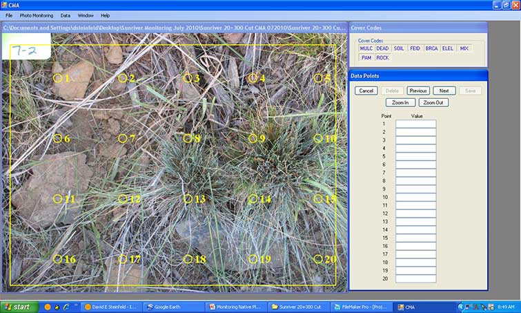
Figure 6-6 | The CMA program reduces field time
Using the CMA program for determining soil cover and/or species cover, each quadrat photo is overlain with a 20-point grid that is randomly placed. Beginning with the first point, the user determines that point lands on a rock and that cover code is entered. The program moves the recorder to the next point until all 20 points are entered. The cover codes are decided by the recorder. In this example, plant cover was detected along with soil, mulch, and rock cover codes. In this case, three plant species were identified (shown as the abbreviations BRCA, ELEL, and FEID) as discussed in Section 6.3.2.
Floral density can be quantified using the CMA program for describing the quality of pollinator foraging habitat while photographs are evaluated for species cover. In this analysis, the number of flowers of each species of interest are counted within the quadrat frame of each photograph (Figure 6-7). A spreadsheet for this procedure is available here.
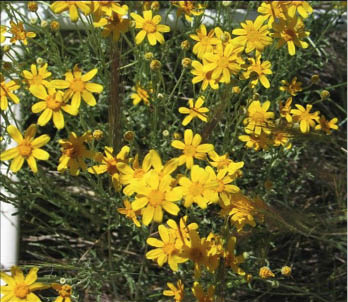
Figure 6-7 | Floral density can be determined using CMA
Floral density can be determined by counting the number of flowers for each species of interest in a quadrat, then evaluated. In this photograph, Oregon sunshine (Eriophyllum lanatum) is the main species that is counted.
Photo credit: David Steinfeld
6.3.3 Species Presence
The Species Presence procedure is an alternative to the Species Cover method of determining whether species are present on the site. While this method still necessitates a person knowledgeable in plant identification in the field, it takes far less time per quadrat because only the presence of a species is recorded. In this method, a fixed frame is placed on the surface of the soil at each quadrat location and the presence or absence a "species of interest" is recorded. Depending on the specific project's success criteria, only species of interest are recorded. Species of interest may include those species that have been seeded, important pollinator supporting species, and undesirable non-native plants. If ecological restoration is a project objective, then all species may be identified.
The size of the fixed frame is based on several factors, such as the growth pattern of the species of interest and the frequency that the species is present on the site. Large frames are not necessary for most grass and forb plant communities. The 1-square-foot frame used for the Soil Cover and Species Cover procedures may suffice (the tall grass prairie systems may be an exception, requiring larger frames). Larger native woody species and undesired weedy species are often measured in quadrats with an area of 1 square meter. This size of quadrat can accommodate the patchy distribution that weedy species frequently display and, when extrapolated, can create a fair representation of the plant species' frequency across the project site. An Excel workbook with field forms and a data analysis package is available here for this procedure.
6.3.4 Plant Density
Trees, shrubs, and wetland plants are typically established from containerized plants grown in nurseries and planted at a specified density depending on the project objectives. Monitoring the density of live plants after they are planted is important to determine how many plants have survived and whether the site will need to be replanted.
The quadrat in this procedure is a circular plot with a specified radius. For trees and shrubs, it is recommended a 1/100 acre plot be used, which has an 11.7-foot radius and covers 436 ft2. A staff is placed at the plot center and a tape or rope is stretched 11.7 feet. While one person holds the staff, the other walks the circumference of the plot and counts the number of plants of each species within the quadrat. This information is recorded on a spreadsheet, such as that shown in the form available in the Native Revegetation Resource Library. This spreadsheet summarizes the total plants per acre and the number of plants per acre by species. Note: for linear sampling areas, only one quadrat is placed randomly within the transect.
Plant density monitoring that is used to determine survival rates are called survival surveys and these are usually conducted six months to a year after planting. If the site is planted in fall or spring and monitoring occurs the following fall, the results are referred to as the "first year survival." Plant density monitoring thereafter is referred to as the years after planting (e.g., third year sampling is "third year survival").
6.3.5 Plant Attributes
This procedure can be used to assess plant growth responses to determine how well plants are growing or whether DFC targets pertaining to growth targets were met. Typically, only sensitive areas, such as visual corridors or wetlands, have stated growth targets. This procedure might have limited applicability to most revegetation projects.
Any part of a plant can be measured for growth, and the selection of an attribute is dependent on the species being sampled. Common attributes include the following:
- Total height—trees and most shrubs
- Last season's leader length—most trees
- Stem diameter—shrubs and trees
- Crown cover—shrubs, forbs, and grasses
Total height is typically measured from the ground surface to the top of the bud. If the plant has several leaders (or tops), the most dominant leader is used for measurement. Last season's leader growth can be observed in most tree species. For conifers, leader growth is measured from the last whorl of branches to the base of the bud. Comparing leader growth from year to year can indicate whether plants are healthy and actively growing.
Stem diameter is also used to measure trees and shrubs. In this method, the basal portion of the plant is measured with calipers at the ground surface. Another attribute is crown cover, which is more conducive to spreading plants, such as shrubs. A large frame with grids or points is placed over the plant to obtain an aerial coverage.
Attributes for shrub and tree species uses the sampling layout and design described for plant density (Section 6.3.4) and focuses only on those species of interest that have been identified in the revegetation plan. If there are many plants of a species of interest in a quadrat, only five plants are measured. An unbiased way to select which plants of each species to monitor is to sample those plants closest to the plot center. If there are not enough plants in the quadrat to sample, then the nearest plants outside of the quadrat are sampled. The measurement for each plant is recorded on a field data sheet, available here. Note: for linear sampling areas, only one quadrat is placed randomly within the transect.
6.3.6 Sampling Unit Design
The shape of the sampling unit determines how quadrats are laid out. Procedures have been developed for linear sampling areas, such as long roadsides; rectilinear sampling areas for rectangular-shaped areas such as restored borrow areas; and dispersed sampling areas, which are revegetation areas that are in patches or clumps. These three sampling designs are described below, as well as how to calculate the minimum number of quadrats to obtain an accurate representation of the sampling unit.
Linear Areas
Linear areas, such as cut slopes, fill slopes, and abandoned roads, are sampled from equally spaced transects placed along the entire length of the sampling unit. Each transect has varying numbers of quadrats, depending on the length of the transect. When the sampling unit is uniform in width, each transect will have an approximately equal number of quadrats; when the width of the revegetation unit is variable, there will be an unequal number of quadrats per transect. In either case, each transect is treated as the primary experimental unit instead of the quadrat (the primary experimental unit in this report is either the transect, quadrat, or dispersed area and is the unit for which statistical analysis is conducted).
Figure 6-8 shows a typical sampling design for a linear area. In this example, the sampling unit included only those portions of the cut slope that were seeded; it did not include road shoulders or the ditch line. For statistical analysis, the number of transects (n) to collect was estimated to be 20 based on pre-monitoring data. Spacing the 20 transects equally along the sampling unit was calculated by dividing the total length of the sampling unit by the number of transects to obtain the distance between transects (3,100/20 = 155 feet). Locating the first transect is done in an unbiased way by generating a random number between 1 and 155. A random numbers table is available here.
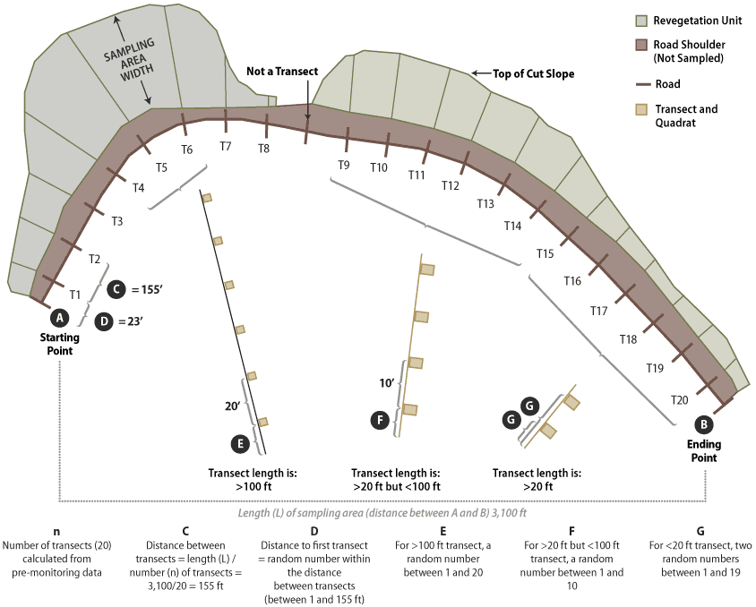
Figure 6-8 | Linear Areas
Linear sampling areas are long units with varying widths. Road cuts, fills, and abandoned roads typically fit this sampling design. The design of linear sampling areas uses a series of equally spaced transects with uniformly spaced quadrats within each transect. The distance between quadrats varies by the length of the transect. Transects longer than 100 feet have 20 feet of spacing between quadrats (T4 through T6), transects between 20 and 100 feet have 10 feet between quadrats (T9 through T14), and transects less than 20 feet long have two randomly placed quadrats (T15 through T20).
Transects are laid out by establishing a line, typically a measuring tape, perpendicular to the edge of the road. The transect begins at the edge of the road beyond the ditch line and where seeding or other treatments were conducted. Each transect contains a series of quadrats spaced as follows:
- <20 foot transect length—For transects where lengths are less than 20 feet, two quadrats are placed. Two random numbers are generated between the numbers 1 and 19. These numbers indicate the location of each transect.
- >20 foot and <100 foot transect lengths—For transects where lengths are between 20 and 100 feet, quadrats are placed at 10-foot intervals. The distance to the first quadrat is based on a random number between 1 and 10 feet.
- >100 foot transect lengths—Long transects have 20 feet between quadrats. The distance to the first quadrat is based on a random number between 1 and 20 feet.
Rectilinear Areas
When sampling units are more elliptical or rectangular in shape, or composed of several large irregular polygons, the sampling design is based on a rectangular grid of quadrats systematically located with a random starting point. Figure 6-9 illustrates an example of such a sampling design. Notice that this design is different from the linear sampling design in that there are no transects. The quadrat in this sampling design is the primary experimental unit, not the transect.
To determine the grid spacing (E) for the quadrat locations, the area of the sampling unit is calculated from maps, and the number of quadrats to be sampled (n) is determined from pre-monitoring data. The following equation gives the length of each side of a square grid (E):

For example, the sampling unit in Figure 6-9 covers 4,262 ft2 and it has been determined from pre-monitoring data that approximately 20 quadrats are necessary to attain the statistical sampling requirements for this sampling unit. The equation indicates that each side (E) of the grid is 14.6 feet:

A starting point of the grid is arbitrarily located in any corner of the study area. To avoid biasing the placement of the quadrats, the corner of the grid is shifted by assigning random numbers to the x and the y coordinates, as shown in Figure 6-9. This is called a systematic design with a random start. It provides equal likelihood that any point in the study area is included in the sample unless there are obvious systematic patterns in the site, such as planting rows. In this example, the random number shifts were 11 feet in the horizontal direction and 4 feet in the vertical direction.
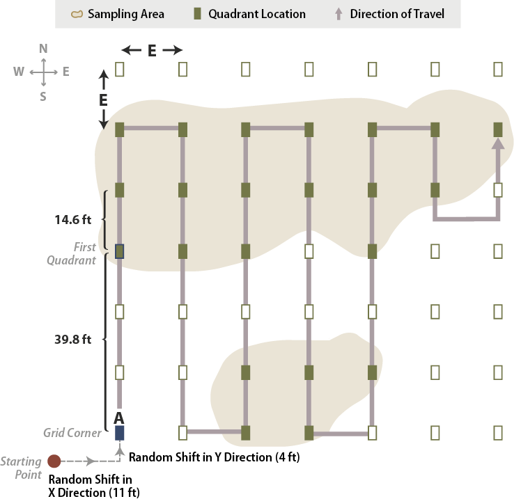
Figure 6-9 | Rectilinear sampling areas
For rectangular or elliptical sampling areas, a grid composed of quadrats is used. The length between grid cells (E) becomes the standard distance between quadrats for this sampling unit. In this example, E = 14.6 feet. To avoid bias, the x and y axes of the grid were randomly offset from the starting point by 11 and 4 feet to a new, random starting point (A). Then 39.8 feet was measured to the first quadrat. The monitoring team follows compass or GPS bearings to locate all quadrats.
The monitoring team locates the random starting point in the field and measures 39.8 feet (10.6 + 14.6 + 14.6 = 39.8) north to the first quadrat. From that quadrat, they measure 14.6 feet north to the second quadrat. After they collect data from the last quadrat in that line, they travel east 14.6 feet to locate the next plot. This system of sampling continues in this fashion until the entire area has been sampled.
Dispersed Areas
When sampling units occur as small, distinct areas, a two-stage sampling design is recommended. The first stage is to determine which dispersed areas to sample, and the second stage is to determine how to sample within each selected area. For the first sampling stage, it is suggested that a minimum of 20 dispersed areas be monitored within each revegetation unit. If there are 20 dispersed areas or fewer, then all dispersed areas are sampled. If there are more than 20 areas, then sampling is conducted with one of two sampling designs. For dispersed areas that are mapped, the systematic sampling design is used. If the dispersed areas are small or are not mapped, then a grid sampling design is used. Both sampling designs are described in more detail below. These areas include planting islands and planting pockets. In most cases, the grid sampling method is recommended.
Systematic Sampling of Dispersed Areas
First Stage
The systematic sampling method of dispersed areas assumes that the dispersed areas have been mapped. The dispersed area in this method is the experimental unit. In this approach, the dispersed areas are numbered sequentially by progressing from one dispersed area to the next closest dispersed area. Determination of the number (n) of dispersed areas to sample is presented in Section 6.3.6, see Sample Size Determination. Odd or even-numbered dispersed areas are selected based on a random number using the RANDBETWEEN function. For example, if there were 40 dispersed areas (N) but only 20 dispersed areas needed to be sampled (n), then 50 percent of the dispersed areas would be sampled (n/N). A random number using RANDBETWEEN (1, 2) is used. If the function returns a "1," the odd-numbered dispersed areas are selected; if 2, then the even numbered areas are selected. Figure 6-10 provides a schematic depiction of such a design.
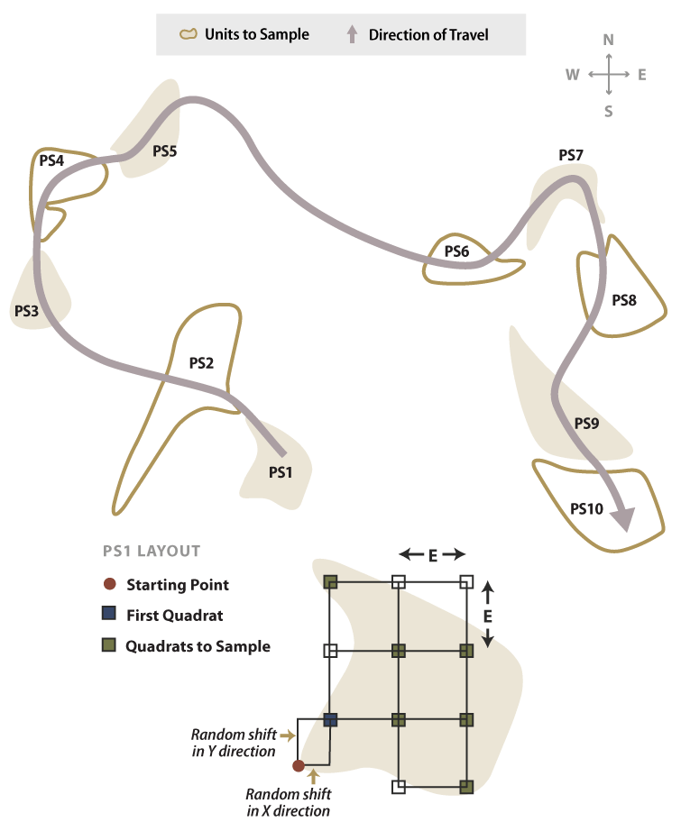
Figure 6-10 | Systematic sampling of dispersed areas
A systematic sample of dispersed areas, shown in this example, is based on 50 percent sampling (the pink areas). Alternating dispersed areas were sampled. Quadrats were located in each sampling unit by first locating a starting point and then measuring off random x and y offset coordinates to locate the first quadrat of the sampling grid.
Second Stage
Once the dispersed areas have been selected, the layout of quadrats within each dispersed area is determined. A grid-based sampling design is used. To determine the grid spacing (E) for the quadrat locations, determine whether the size of the dispersed area is >1,600 ft2 or <1,600 ft2 (1,600 ft2 is a 40-by-40-foot area). Depending on the sample size, the number of quadrats will be as follows:
- Less than 1,600 feet—four quadrats
- More than 1,600 feet—eight quadrats
Using the following equation, the grid sides (E) are determined where n = 4 or 8 (depending on the size of the dispersed area) and the area is the estimated size of the dispersed area.

This calculation is made for each dispersed area. To avoid biasing the placement of quadrats, a predetermined starting point is made (e.g., the northwest corner of each dispersed area). Random x and y coordinates are generated for each dispersed area that is within the predetermined length of the square grid (E). The corner of the grid is placed at this point and oriented north. The location of the first quadrat is x and y feet from the starting point, as shown in Figure 6-10.
For the plant density and plant attribute procedures, only one quadrat is randomly located within each dispersed sampling area. The location is determined by assigning the RANDBETWEEN random number function to the number of quadrats determined for the dispersed area. The random number that is generated is the quadrat selected for sampling.
Grid Sampling of Dispersed Areas
First Stage
A grid sampling design is used on projects where dispersed areas have not been mapped and there are more than 30 areas. This sampling design is used on projects where dispersed areas are numerous and the sizes of the areas are small. In this sampling design, a grid is placed over the revegetation unit, as shown in Figure 6-11, and the dispersed area nearest to a grid crossing is selected for monitoring. One quadrat is randomly placed in each dispersed area and this becomes the experimental unit.
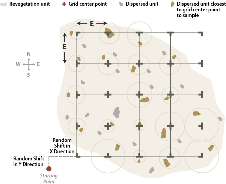
Figure 6-11 | Sampling dispersed areas with an offset grid
A systematic sample of dispersed areas, shown in this example, is based on 50 percent sampling (the pink areas). Alternating dispersed areas were sampled. Quadrats were located in each sampling unit by first locating a starting point and then measuring off random x and y offset coordinates to locate the first quadrat of the sampling grid.
Determining the grid cell dimensions (E) is accomplished by using the following equation:
The grid is laid out in an unbiased manner by locating a starting point just outside the revegetation unit and assigning random numbers as offsets for the x and y coordinates. The corner of the grid is placed at the x and y offset point and oriented north. At each grid crossing, the closest dispersed area is selected for monitoring. If there are no dispersed areas found within half the distance between grid centers ( E / 2 ), then the monitoring team moves on to the next grid center.
Second Stage
Since the dispersed areas are small (e.g., planting pockets, planting islands, benches), all measurements for seedling density and seedling attributes may be sampled within each dispersed area. For other procedures, such as soil cover, species cover, or species presence procedures, one quadrat is located randomly in the dispersed area.
Sample Size Determination
This section covers how to take pilot data to determine the number of experimental units (transects or quadrats) needed to statistically monitor a sampling unit. It is important to note that an alternative to taking pilot data is to simply to sample a minimum of 20 primary experimental units per sampling unit. For example, for a linear sampling area, 20 transects are laid out; for rectilinear areas—20 quadrats; and for a dispersed area sampling design—20 dispersed areas). Twenty primary experimental units will provide adequate data to accurately estimate means and confidence limits and to understand the uncertainty (i.e., width of confidence intervals). The risk is that, in some cases, the intervals may be too wide to provide meaningful estimates, which means that more samples would be needed, requiring revisiting of the sampling unit. Generally, if data are moderately variable and symmetrically distributed, 20 experimental units will often be adequate (personal communication: John Kern, Kern Statistical Services Inc., February 10, 2017). The following section is intended for projects where a more exact sample size, using pilot data, is desired to achieve the precision requirements of the monitoring plan.
Sample size determination methods are tailored to the monitoring objectives and sampling area design. This section outlines four sampling methods: (1) comparing means with DFC target for linear area sampling design, (2) comparing means with DFC targets for rectilinear sampling area design, (3) comparing means with DFC target for dispersed areas, and (4) determining sample size for comparing treatment areas.
Comparing Means with DFC Targets—Linear Sample Size Determination
To calculate the minimum sample size for linear sampling areas the expected sample mean and the range in values are approximated. A visual estimate of the mean and the range of values may be adequate. For more precise estimates, four transects are sampled in the field to establish estimates of the mean and range of values.
The following is a quick method to determine the number of transects to sample based on pre-monitoring data collection:
- Driving the entire revegetation unit and noting extremes in vegetation
- Finding four areas that represent the extremes and laying out a transect in each area
- Randomly placing two quadrats within each transect to collect data on the attribute of interest (e.g., percent ground cover)
- For each transect, averaging the quadrat values (four averages)
- Calculating the average of the four transect averages and the range (difference between highest and lowest values of the four averages)
- Applying the range and the average to the following equation to obtain the minimum number of transects needed to monitor the revegetation unit (equation based on a sample size of 20 percent of the true population value with 90 percent confidence):
n = (0.838 * Range)2 / (0.2 * x̄ )2
The number of transects (n) obtained from this quick assessment is used to determine the layout of the monitoring design, as described in Section 6.3.5.
Example: Suppose that monitoring is to be conducted along a road cut to determine the percentage of soil cover. The monitoring objective is to estimate mean percent cover to within 20 percent of the true population value with 90 percent confidence. Four transects that represent a range in conditions are laid out within the revegetation unit. These transects do not need to be located randomly but rather can be sited to capture the range of values observed in the sampling unit. It is better to over-estimate the range of values, as this will tend to result in a conservative estimate of the sample size. The data set and equation are shown in Figure 6-12.
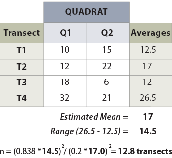
Figure 6-12 | Determining the number of transects using pilot data
Example of how to calculate the number of transects needed, based on the pre-monitoring data set.
Using the equation presented above, an estimated 13 transects were calculated for a minimum sample size.
Comparing Means with DFC Targets—Rectilinear Sample Size Determination
When a grid of quadrats is to be implemented, the sample size calculations use quadrat measurements as opposed to the transect averages that were used in linear sampling areas. The steps involved in calculating the number (n) of quadrats are as follows:
- Visiting the entire revegetation unit and noting extremes in revegetation
- Finding four areas that represent the extremes and laying out a transect in each area
- Randomly placing two to three quadrats within each transect to collect data on the variable of interest (e.g., percent ground cover)
- Averaging the quadrat values (eight quadrat values to average)
- Calculating the range of all eight samples (difference between highest and lowest values)
- Applying the range and the average to the following equation to obtain the minimum number (n) of transects needed to monitor the revegetation unit:
n = (0.838 * Range)2 / (0.2 * x̄ )2
Example: Using the data from the previous example (Figure 6-12), the eight quadrats would be averaged (instead of four transect averages being averaged). While the mean in this example remains 17, the range has spread to 26 (maximum 32 minus the minimum 6). The number of quadrats to sample would be 41:
n = (0.838 * 26)2 / (0.2 * 17.0 )2 = 41.126
Comparing Means with DFC Targets—Dispersed Area Sample Size Determination
Systematic Sampling Method: The systematic sampling method is used when the dispersed areas are mapped (see Systematic Sampling of Dispersed Areas). The primary experimental unit in this design is the dispersed area. The number of quadrats to sample is estimated by following these steps:
- Finding four dispersed areas that represent the extremes of the attribute of interest
- Randomly placing two quadrats within each dispersed area to collect data on the attribute of interest (e.g., percent ground cover)
- For each dispersed area, calculating the average of the four dispersed areas' averages and the range
- Applying the range and the average to the following equation to obtain the minimum number of dispersed areas needed to monitor in a revegetation unit (equation based on a sample size of 20 percent of the true population value with 90 percent confidence):
n = (0.838 * Range)2 / (0.2 * x̄ )2
An example of the data set and equation are shown in Figure 6-12. Note: substitute "dispersed area" for "transect" in the first column heading.
Grid Sampling Method: The grid sampling method is used for revegetation units that have small dispersed areas that have not been mapped (see Grid Sampling of Dispersed Areas). Since only one quadrat is in a dispersed area, the quadrat becomes the primary experimental unit. The number of quadrats to sample is estimated by following these steps:
- Visiting a range of dispersed areas and selecting eight dispersed areas that represent extremes of the attribute of interest
- Randomly placing one quadrat in each dispersed area and collecting data on the attribute of interest (e.g., percent ground cover)
- Calculating the average and range in values
- Applying the range and the average to the following equation to obtain the minimum number (n) of dispersed areas to sample:
n = (0.838 * Range)2 / (0.2 * x̄ )2
Example: Using the data from the previous example (Figure 6-12), the eight quadrats would be averaged (instead of four transect averages being averaged). While the mean in this example remains 17, the range has spread to 26 (maximum 32 minus the minimum 6). The number of quadrats to sample would be 41:
n = (0.838 * Range)2 / (0.2 * x̄ )2
Comparing Means among Treatment Groups—Sample Size Determination
When determining the sample size for comparing treatment differences (Section 6.3.7), it is not necessary to differentiate between linear, rectilinear, or dispersed sampling area designs. Sample size determinations follow these steps:
- Reviewing each treatment area to be compared. These can be different revegetation units or different types of revegetation treatments.
- From each treatment area, collecting data from two transects with each transect consisting of two quadrats. These should represent a range of extremes for a total of four transects.
- Determining the range between the low and high quadrat values.
- Determining delta (also represented by Δ). Delta defines the level of significance that is needed for monitoring, or the meaningful difference in measurement output. For example, calculating bare soil at 1 percent difference in means would be unimportant, that is, the difference between 8 and 9 percent bare soil is too fine a distinction to make. A 5 percent difference might be important if the amount of data that is needed to be collected was not great. More than likely, a 10 percent difference (e.g., the difference between 10 and 20 percent bare soil) would be an acceptable delta value for bare soil cover. It is important to note that the smaller the delta value, the more samples that need to be collected.
The number of transects (n) can be calculated using a simplified equation:
n = 15.68 / (Δ * 2.059 / Range)2
The number of transects determined from these calculations are applied equally to the two (or more) areas being compared. This equation assumes that tests will be conducted at the delta level of significance and that there will be a difference detected at or greater than an 80 percent probability.
Example: A test was set up to determine whether a commercial product could increase plant cover by at least 10 percent one year after application, as advertised. In one area, the product was applied and in another similar area, it was not. To determine the number of transects to install in each area, a year after application, two transects were set up in the treated area and two transects in the untreated area. From the quadrat readings, the range in percent vegetative ground cover values was found to be 22. Assuming a delta level of significance of 10 percent (important to be able to detect a difference in 10 percent cover with at least 80 percent probability), the following number of transects required for each treatment area were determined to be 18:
n = 15.68 / (10 * 2.059 / 22)2 = 17.9 transects
In general, using the simple equation provided here, and possibly adding 10 to 20 percent additional samples as a level of conservatism, is a reasonable approach.
6.3.7 Analyze Data
This section provides statistical methods for analyzing data collected for all monitoring procedures described in the previous section. There are three types of analysis based on the objective of the area being monitored:
- Compliance—Determine whether DFC targets were met
- Treatment differences—Determine whether there were differences between treatments or changes between years
- Trends—Determine the degree of vegetation or soil cover change over time
Only one of these procedures is selected for an analysis depending on the monitoring objective used. These procedures use confidence intervals to determine the statistical significance of the monitoring data set.
Analysis of Compliance
The objective behind most monitoring is to answer these three questions:
- Was the project successful?
- Were DFC targets met?
- Were the commitments made to the community and those described in planning and compliance documents and reports met in terms of protecting soil, reestablishing native vegetation, and maintaining or improving pollinator habitat?
To answer these questions, the means of the attribute data of interest (e.g., bare soil, species presence) are compared with the DFC targets. For example, a project has a DFC target of at least 70 percent soil cover on a road cut near a live stream one year after road construction. Using the soil cover procedure, data are collected on 20 transects and a mean of 81 percent soil cover is determined. At this point, the designer might conclude that the targets were met. From a statistician's point of view, however, the data displayed in this context is inconclusive because the variability of the soil cover in the sampling unit is not known or cannot be accounted for. In other words, how good is the number? Is it really depicting what is happening on the site? If another person were to use the soil cover procedure in the same sampling unit but at a different spot, would the soil cover be exactly 81 percent? This is highly unlikely because of the high variability of soil cover.
Confidence intervals provide a means of predicting, at a chosen level of certainty, whether the soil cover value collected anywhere in the sampling unit will be within a stated range. Confidence intervals are an alternative to saying, "we think the soil cover at any point in the sampling unit will be around 81 percent." Using confidence intervals, it can be said instead that, "we are 90 percent confident that if data collection was repeated at this site 10 times, 9 out of 10 times the average soil cover estimate would be within our confidence limits." If a higher confidence level is desired (most scientists working in health fields want to be more certain), confidence intervals can be based on 95 percent or even 99 percent certainty. In this case, the confidence interval would be much wider.
The data sets from very different revegetation units are shown in Figure 6-13 to convey the concept of confidence intervals. While both data sets have the same mean of 81 percent soil cover, the confidence intervals are very different. Data set A was taken at a site with very uniform soil cover, while data set B had much more variability. For both data sets, a 90 percent confidence interval is desired. Notice that the confidence interval for data set B is much wider than data set A since it has greater variability.
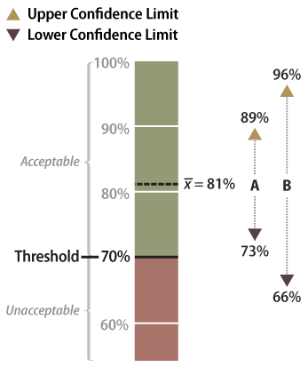
Figure 6-13 | Example data analysis results
Data set A has an upper confidence limit of 89 percent and a lower confidence limit of 73 percent. Since the lower confidence limit is above the target, or threshold, of 70 percent, it can be stated with 90 percent confidence that the target was met. Data set B has a wider confidence interval and a lower confidence limit of 66 percent, which is below the target. In this case, there is uncertainty at the 90 percent confidence limit that the target was met.
With confidence intervals, it can be said with greater certainty whether the DFC target or threshold of 70 percent soil cover was met. It can be stated with 90 percent confidence that data set A met the target because the lower confidence limit (73 percent) is above the target of 70 percent. Alternatively, data set B poses some problems. It cannot be said with 90 percent confidence that the average is above the threshold of 70 percent because the lower confidence limit of data set B is 66 percent, or 4 percent below the threshold. The designer might argue that, because the mean is above the target, the target was met. To statisticians, however, the fact that the lower confidence interval is below the stated target indicates a fair amount of uncertainty. They would have to obtain more data or change how confident the prediction is before they could be certain the DFC target was met.
Calculating Confidence Intervals
Workbooks are available in the Native Revegetation Resource Library to calculate confidence intervals depending on the sampling unit design (Section 6.3.6):
- Linear sampling design—Select this Excel workbook for linear sampling designs.
- Rectilinear sampling design—Select this Excel workbook for rectilinear sampling designs.
- Dispersed sampling design—For this sampling design, there are two workbooks to choose from. If a grid sampling design was used, this Excel workbook is used, and if a systematic sampling design was used, this workbook is used.
Interpreting Confidence Intervals for Compliance
Confidence intervals, as stated previously, are used to evaluate the success of a revegetation project relative to a specified DFC target. For example, an objective of a revegetation project was to establish at least 65 percent total cover over the soil to protect against surface erosion. Or stated another way, the objective was that no more than 35 percent bare soil would be exposed one year after revegetation treatments were applied. During monitoring, it was found that the lower confidence level was 23.8 and the upper confidence level was 30.8, both below the target of 35 percent. It could be said with a 90 percent level of confidence that the objectives were met. But what if the confidence interval was either above the target or straddled the target?
Figure 6-14 shows four possible scenarios for confidence intervals that may be encountered. Scenario A is a case in which the data supports the conclusion at 90 percent confidence that the project met the target. Scenario B did not meet the target because the lower confidence limit was above 35 percent bare soil.
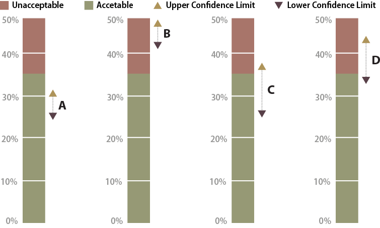
Figure 6-14 | Possible scenarios when comparing targets to confidence intervals
Four possible scenarios that can be encountered when comparing targets to confidence intervals. Confidence interval A is clearly acceptable, whereas confidence interval B is clearly unacceptable. Uncertainty arises when the lower confidence limit is acceptable but the upper confidence limit is unacceptable. This is shown in cases where the mean is in the acceptable range (C) and in the unacceptable range (D).
Scenario C is a case where the mean meets the target, but the upper confidence limit is above the target. It cannot be said with 90 percent confidence that the targets were met. At this point it might be asked how important it is to know whether the target was met. If the site directly influences a live stream, it might be very important. However, if there are no streams nearby, it might suffice to report that there was some uncertainty whether the target was met. If it is determined that more certainty is needed, more data must be collected.
Scenario D is a case where the mean does not meet the target, but the lower confidence limit is below the target of 35 percent bare soil. One might state that this project did not meet the target, but this still could not be stated with 90 percent confidence. In this scenario, more transects could be taken to narrow the confidence interval and hope that the results do not straddle the target.
Another option for Scenarios C and D might be to implement measures to decrease the amount of bare soil. This could include more seeding or application of mulch. The site would be resampled after an interval of time to determine whether the DFC target had been met.
Analysis of Treatment Differences
There may be opportunities to compare the effects of different revegetation products or methods on plant establishment and growth using monitoring data. Some of these opportunities will be planned (e.g., trying a new product), and some will be mistakes (e.g., inadvertently doubling the rate of mulch application). Planned or unplanned, when different revegetation activities have occurred within a revegetation unit, monitoring can be designed to assess whether there is a different vegetative response between those activities or treatments. The monitoring design outlined in this section will not replace a well-designed study or experiment; it is suggested that if more conclusive results of treatment differences are desired, a study would be designed with statistical oversight. An Excel workbook is available in the Native Revegetation Resource Library for this analysis.
The confidence interval concept is applied in this subsection to determine differences between new revegetation treatments (new treatments) and routine revegetation methods (standard treatments). Three possible outcomes are possible when new treatments are compared to standard methods: (1) the new treatment results in a favorable increase in the measured parameters over the standard treatment (positive difference), (2) the new treatment results in a decrease (negative difference), or (3) there is no positive or negative difference (no difference). Using confidence intervals, it is possible to determine which of these outcomes is statistically supported for any monitoring data set. In this method, the means and variance of means are calculated for both the new treatment and standard treatment and a confidence interval is calculated for the certainty of the treatment differences.
The following example demonstrates how a confidence interval is determined and how it can be used to interpret two data sets. During a hydroseeding operation, it is discovered that fertilizer was mistakenly applied at twice the normal rate in one area. This area was staked in the field when the realization was made and visited by the project team a year later. Some on the team believed that there was more vegetative ground cover where fertilizer was doubled; others felt that there was less. One or two on the team did not believe they could make either call. Since monitoring was going to occur a few weeks later, they decided to design a monitoring procedure to answer the question, "Was there a positive, negative, or no response of vegetative ground cover to the application of additional fertilizer?"
Within the framework of monitoring that was already scheduled for this revegetation unit, a monitoring strategy was developed. The species cover procedure was used (Section 6.3.2) along with the linear sampling design since this was a road cut (Section 6.3.6). Each treatment area was considered a separate sampling unit, and monitoring of each treatment area took place independently of the others. The data from each treatment area was recorded in the Species Cover spreadsheet (see Species Cover Monitoring Procedure workbook) to obtain means and variance of means. These values were then entered into the Comparing Treatment Differences Monitoring Procedure spreadsheet to obtain confidence intervals.
The results of this analysis showed that the standard rates of fertilizer had an average vegetative ground cover of 33 percent as compared to 62 percent for double the fertilizer rate. While this looks like an obvious difference, how certain could the team be? In this example, the confidence interval (at 90 percent confidence) showed that additional fertilizer significantly increased vegetative ground cover. This can be shown graphically in Figure 6-15. The doubled fertilizer treatment increased ground cover a minimum of 16 percent (lower confidence interval) over the standard treatment to as much as 42 percent ground cover (upper confidence limit).
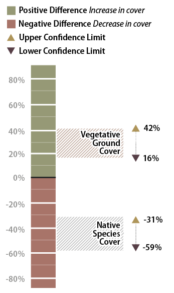
Figure 6-15 | Interpreting results with confidence intervals
In the example presented in the text, confidence intervals are used to answer: (1) how vegetative ground cover responds to 2X the fertilizer rate, and (2) how native species cover responds to 2X the fertilizer rates. The confidence interval collected for the first question was found to be positive, indicating that vegetative ground cover responds positively to twice the fertilizer. The confidence interval for the data set collected for the second question was negative, indicating that native species cover responded negatively to more fertilizer.
The team accepted these results and commented that fertilizer rates should be increased for future projects. One member posed the question, "We might have achieved better vegetative cover on this site during the first year, but how did additional fertilizer affect the native species cover?" Since the monitoring team was still on the project site, they resampled the two areas using the species cover procedure (Section 6.3.2). In this procedure, native and non-native annuals and perennials were recorded at each quadrat. Confidence intervals were determined for each treatment for native perennial cover and they learned, in this case, that additional fertilizer had a negative effect on the establishment of native perennial cover (Figure 6-15). But what if the upper confidence interval in this example had been positive and the lower confidence interval had been negative? In this case, it would have to be concluded that there was no difference between treatments at 90 percent confidence.
Analysis of Trends
The last of the three objectives for roadside monitoring is assessing trends, or the degree that attributes, such as vegetative or soil cover, change over time. One of the main reasons to perform this type of monitoring is to understand how plant growth or successional patterns change. Many monitoring procedures employ permanent monitoring plots or transects that can be repeatedly and accurately revisited for sampling. This approach does not work as well for roadside monitoring however, because of the hazards to road maintenance personnel and to the public of placing permanent stakes in road corridors. In addition, permanent markers are often hard to relocate years later or can move due to the instability of steep cut and fill slopes. In this section, a statistical analysis that does not entail locating and resurveying of exact quadrats is offered. An Excel workbook is available here for this procedure.
The confidence interval approach is applied in this section to determine if there are differences in attributes from one sampling date to another. Three outcomes are possible when comparing data from one sampling date to the next: (1) attributes have increased since the last sampling period (positive difference), (2) attributes have decreased since the last sampling period (negative difference), or (3) either there was no change in attributes or the number of samples was inadequate to detect the amount of change that occurred. Using confidence intervals, it is possible to make statistically valid statements regarding the observed outcomes.
The following example demonstrates how confidence intervals are determined and how they are used to interpret data collected on different sampling dates. Members of the project team believed that California brome (Bromus carinatus; BRCA5) was a short-lived species; that it established well after seeding but by the fifth year it had very little presence on most sites. They also believed that Idaho fescue (Festuca idahoensis; FEID) started out slowly but gained dominance over time. The team felt that by understanding these trends they might develop a better seed mix for sites like the ones they were monitoring. The question they posed was: "Is there a positive, negative, or no difference in the cover of California brome and Idaho fescue from the first year to the fifth year after seeding?"
This question necessitated the use of the Species Cover procedure (Section 6.3.2) since dominance was being expressed as percent crown cover for each species. Linear Sampling Design was used for both monitoring dates because the sampling unit was a long cut slope. The data from each sampling date for California brome and Idaho fescue was entered into the spreadsheet shown in the Species Cover spreadsheet (see Species Cover Monitoring Procedure workbook) to obtain means and variance of means. These values were then entered into the spreadsheet shown in the Analyzing Trends Monitoring Procedure workbook to produce confidence intervals for comparison. Data entry was also conducted in the same manner for Idaho fescue.
The results of this analysis showed that California brome had an average crown cover of 35 percent in 2001 but decreased to 27 percent in 2006, five years later. Was this a statistically significantly difference? Using confidence intervals, it was determined that the means were not statistically different at 90 percent confidence. This can be shown graphically in Figure 6-16. Because the upper confidence limit was positive and the lower was negative, the team could be 90 percent confident that crown cover did not increase from 2001 to 2006. Alternatively, Idaho fescue did show an increase in mean crown cover from 2001 to 2006. This increase was found to be significant because both the upper and lower confidence limits were positive. The team could be 90 percent confident that there was a true increase in crown cover.
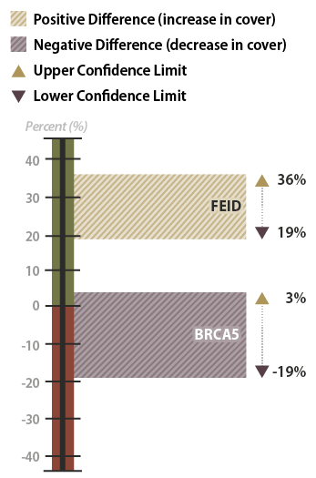
Figure 6-16 | Example results with confidence intervals
In the example, confidence intervals were used to determine whether California brome (BRCA5) and Idaho fescue (FEID) increased, decreased, or stayed the same from 2001 to 2006. The percent crown cover of California brome was found not to have changed during this period because the lower confidence limit was negative and the upper confidence limit was positive. The confidence interval for the Idaho fescue showed an increase between 2001 and 2006. Since the upper and lower confidence limits were positive, the differences in the means between sampling dates were significant at 90 percent confidence.